A from-scratch implementation of Kolmogorov-Arnold Networks (KAN)…and MLP

Kolmogorov-Arnold networks (KAN) were recently introduced in [1] and have already sparked significant interest in the AI community. They offer the potential for both accuracy and interpretability, although some speculate that they might not easily adapt to massively parallelized computation architectures like GPUs.

KANs emerge when edge functions are nonlinear in their inputs and can be expressed as a weighted sum of B-splines. Conversely, when edge functions are linear, the architecture simplifies to the traditional Multi-Layer Perceptron (MLP).

Only time will tell whether KANs will be widely adopted by the AI community. Nonetheless, in this post, we use KANs as a nice opportunity to implement them from scratch in simple Python (no PyTorch / TensorFlow: just some good old numpy!).

We actually construct a general-purpose fully-connected feed-forward network that can be instantiated into either KAN or classic MLP as sub-cases. This exercise also serves as a valuable way to review various concepts related to backpropagation in general feed-forward networks.

The code discussed in this post is available in the GitHub repository [3].

Specifically, all figures can be generated via the Jupyter notebook here.

We emphasize that our goal here is pedagogy, rather than efficiency.

1. A versatile neuron architecture

We start by describing a general neuron structure capable of accommodating both KANs and MLPs as sub-cases.

We call ${\mathbf{x}^{\mathrm{in}}=[x^{\mathrm{in}}_1,\dots,x^{\mathrm{in}}_M]}$ the neuron’s input. Its ${i}$ -th element undergoes a transformation via the parameterized edge function ${\phi(.,\mathbf{w}^i)}$ , where ${\mathbf{w}^i=[w^i_1,\dots,w^i_K]}$ is the set of learnable weights, resulting in the intermediate variable ${x^{\mathrm{mid}}_i}$ :

$\displaystyle x^{\mathrm{mid}}_i = \phi\left( x^{\mathrm{in}}_i, \mathbf{w}^i \right). \ \ \ \ \ (1)$

Then, the node function ${\sigma}$ aggregates the intermediate variables into the neuron’s output ${x^{\mathrm{out}}}$ :

$\displaystyle x^{\mathrm{out}} = \sigma\left( \mathbf{x}^{\mathrm{mid}}, b \right) \ \ \ \ \ (2)$

where ${b}$ is the neuron’s bias, which is also learnable.

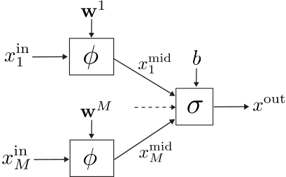
A “loss” function ${\mathcal L}$ , described later on, evaluates the network’s prediction quality against a ground truth. Our goal is to learn the values of weights and biases ${w,b}$ minimizing the loss. To this aim, we evaluate the loss derivative with respect to the parameters and update these via gradient descent. We can then split these derivatives into smaller chunks via chain rule as:

$\displaystyle \frac{\mathrm{d} \mathcal L}{\mathrm{d} w^i_j} = \frac{\mathrm{d} \mathcal L}{\mathrm{d} x^{\mathrm{out}}} \frac{\mathrm{d} x^{\mathrm{out}}}{\mathrm{d} w^i_j}, \qquad \forall \, i,j \ \ \ \ \ (3)$

$\displaystyle \frac{\mathrm{d} \mathcal L}{\mathrm{d} b} = \frac{\mathrm{d} \mathcal L}{\mathrm{d} x^{\mathrm{out}}} \frac{\mathrm{d} x^{\mathrm{out}}}{\mathrm{d} b}. \ \ \ \ \ (4)$

We leave the term ${\frac{\mathrm{d} \mathcal L}{\mathrm{d} x^{\mathrm{out}}}}$ unspecified for now, as it will be provided by other neurons downstream via backpropagation, given its dependence on the network structure down the line.

On the other hand, the terms ${\frac{\mathrm{d} x^{\mathrm{out}}}{\mathrm{d} b}, \frac{\mathrm{d} x^{\mathrm{out}}}{\mathrm{d} w^i_j}}$ only depend on quantities internal to the neuron. Conveniently, chain rule breaks down ${\frac{\mathrm{d} x^{\mathrm{out}}}{\mathrm{d} w^i_j}}$ into:

$\displaystyle \frac{\mathrm{d} x^{\mathrm{out}}}{\mathrm{d} w^i_j} = \frac{\mathrm{d} x^{\mathrm{out}}}{\mathrm{d} x^{\mathrm{mid}}_i} \, \frac{\mathrm{d} x^{\mathrm{mid}}_i}{\mathrm{d} w^i_j}, \qquad \forall\, i,j \ \ \ \ \ (5)$

For backpropagation purposes, it is also convenient to store the output derivative with respect to the inputs:

$\displaystyle \frac{\mathrm{d} x^{\mathrm{out}}}{\mathrm{d} x^{\mathrm{in}}_i} = \frac{\mathrm{d} x^{\mathrm{out}}}{\mathrm{d} x^{\mathrm{mid}}_i} \, \frac{\mathrm{d} x^{\mathrm{mid}}_i}{\mathrm{d} x^{\mathrm{in}}_i}, \qquad \forall\, i \ \ \ \ \ (6)$

We report below the Python class implementing the general-purpose neuron architecture just described.

import numpy as np

class Neuron:

    def __init__(self, n_in, n_weights_per_edge, weights_range=None):
        self.n_in = n_in  # n. inputs
        self.n_weights_per_edge = n_weights_per_edge
        weights_range = [-1, 1] if weights_range is None else weights_range
        self.weights = np.random.uniform(weights_range[0], weights_range[-1], size=(self.n_in, self.n_weights_per_edge))
        self.bias = 0
        self.xin = None  # input variable
        self.xmid = None  # edge variables
        self.xout = None  # output variable
        self.dxout_dxmid = None  # derivative d xout / d xmid: (n_in, )
        self.dxout_dbias = None  # derivative d xout / d bias
        self.dxmid_dw = None  # derivative d xmid / d w: (n_in, n_par_per_edge)
        self.dxmid_dxin = None  # derivative d xmid / d xin
        self.dxout_dxin = None  # (composite) derivative d xout / d xin
        self.dxout_dw = None  # (composite) derivative d xout / d w
        self.dloss_dw = np.zeros((self.n_in, self.n_weights_per_edge))  # (composite) derivative d loss / d w
        self.dloss_dbias = 0  # (composite) derivative d loss / d bias

    def __call__(self, xin):
        # forward pass: compute neuron's output
        self.xin = np.array(xin)
        self.get_xmid()
        self.get_xout()

        # compute internal derivatives
        self.get_dxout_dxmid()
        self.get_dxout_dbias()
        self.get_dxmid_dw()
        self.get_dxmid_dxin()

        assert self.dxout_dxmid.shape == (self.n_in, )
        assert self.dxmid_dxin.shape == (self.n_in, )
        assert self.dxmid_dw.shape == (self.n_in, self.n_weights_per_edge)

        # compute external derivatives
        self.get_dxout_dxin()
        self.get_dxout_dw()

        return self.xout

    def get_xmid(self):
        # compute self.xmid
        pass

    def get_xout(self):
        # compute self.xout
        pass

    def get_dxout_dxmid(self):
        # compute self.dxout_dxmid
        pass

    def get_dxout_dbias(self):
        # compute self.dxout_dbias
        pass  #self.dxout_dbias = 0  # by default

    def get_dxmid_dw(self):
        # compute self.dxmid_dw
        pass

    def get_dxmid_dxin(self):
        # compute self.dxmid_dxin
        pass

    def get_dxout_dxin(self):
        self.dxout_dxin = self.dxout_dxmid * self.dxmid_dxin

    def get_dxout_dw(self):
        self.dxout_dw = np.diag(self.dxout_dxmid) @ self.dxmid_dw

    def update_dloss_dw_dbias(self, dloss_dxout):
        self.dloss_dw += self.dxout_dw * dloss_dxout
        self.dloss_dbias += self.dxout_dbias * dloss_dxout

    def gradient_descent(self, eps):
        self.weights -= eps * self.dloss_dw
        self.bias -= eps * self.dloss_dbias

Note that a number of derivative terms are not specified, since they depend on the edge and node functions ${\phi,\sigma}$ which have not been instantiated yet. We will do this in the next two sections.

1.1. “Classic” neuron

We now instantiate the general neuron structure into the “classic” one, with linear edge functions ${\phi}$ :

$\displaystyle x_i^{\mathrm{mid}} := \phi(x_i^{\mathrm{in}},w^i) = w^i x_i^{\mathrm{in}} \ \ \ \ \ (7)$

The output variable is obtained by applying the activation function ${\sigma}$ to the sum of intermediate variables and the bias:

$\displaystyle x^{\mathrm{out}} = \sigma\left( \mathbf{x}^{\mathrm{mid}}, b \right) := \sigma\left( b+\sum_{i=1}^M x^{\mathrm{mid}}_i \right). \ \ \ \ \ (8)$

The activation function ${\sigma}$ can be defined, e.g., as ReLU ( ${\sigma(x)=0}$ for ${x\le 0}$ , ${\sigma(x)=x}$ else), sigmoid ( ${\sigma(x)=1/(1+e^{-x})}$ ), or hyperbolic tangent functions.

import math

def relu(x, get_derivative=False):
    return x * (x > 0) if not get_derivative else 1.0 * (x >= 0)

def tanh_act(x, get_derivative=False):
    if not get_derivative:
        return math.tanh(x)
    return 1 - math.tanh(x) ** 2

def sigmoid_act(x, get_derivative=False):
    if not get_derivative:
        return 1 / (1 + math.exp(-x))
    return sigmoid_act(x) * (1 - sigmoid_act(x))

We can now compute all the auxiliary derivatives needed to finally produce the loss gradient via (3), (4):

$\displaystyle \frac{\mathrm{d} x^{\mathrm{mid}}_i}{\mathrm{d} w^i} = x_i^{\mathrm{in}}, \quad \frac{\mathrm{d} x^{\mathrm{mid}}_i}{x_i^{\mathrm{in}}} = \mathrm{d} w^i, \quad \frac{\mathrm{d} x^{\mathrm{out}}}{\mathrm{d} x^{\mathrm{mid}}_i} = \frac{\mathrm{d} x^{\mathrm{out}}}{\mathrm{d} b} = \sigma'. \ \ \ \ \ (9)$

where ${\sigma'}$ is the derivative of ${\sigma}$ .

Now, let’s dive into the code. The NeuronNN class inherits from the Neuron class template and computes the derivatives as described above.

class NeuronNN(Neuron):

    def __init__(self, n_in, weights_range=None, activation=relu):
        super().__init__(n_in, n_weights_per_edge=1, weights_range=weights_range)
        self.activation = activation
        self.activation_input = None

    def get_xmid(self):
        self.xmid = self.weights[:, 0] * self.xin

    def get_xout(self):
        self.activation_input = sum(self.xmid.flatten()) + self.bias
        self.xout = self.activation(self.activation_input, get_derivative=False)

    def get_dxout_dxmid(self):
        self.dxout_dxmid = self.activation(self.activation_input, get_derivative=True) * np.ones(self.n_in)

    def get_dxout_dbias(self):
        self.dxout_dbias = self.activation(self.activation_input, get_derivative=True)

    def get_dxmid_dw(self):
        self.dxmid_dw = np.reshape(self.xin, (-1, 1))

    def get_dxmid_dxin(self):
        self.dxmid_dxin = self.weights.flatten()

1.2. KAN neuron

As described in the seminal paper [1], the peculiarity of Kolmogorov-Arnold Network (KAN) neuron is in the edge function ${\phi}$ , defined as a linear combination of (non-linear) functions ${f_k}$ :

$\displaystyle x^{\mathrm{mid}}_i = \phi\left(x^{\mathrm{in}}_i \right) := \sum_{k=1}^K w^i_k f_k \left(x^{\mathrm{in}}_i\right) \ \ \ \ \ (10)$

Hence, the derivative write:

$\displaystyle \frac{\mathrm{d} x^{\mathrm{mid}}_i}{\mathrm{d} w^i_k} = f_k\left(x^{\mathrm{in}}_i\right), \quad \frac{\mathrm{d} x^{\mathrm{mid}}_i}{x_i^{\mathrm{in}}} = \sum_{k=1}^K w^i_k f'_k\left(x^{\mathrm{in}}_i\right). \ \ \ \ \ (11)$

In [1], it is suggested that the edge functions ${f_k}$ ‘s should be B-spline except for ${f_1(x):=\mathrm{silu}(x)=x/(1+e^{-x})}$ .

from scipy.interpolate import BSpline

def get_bsplines(x_bounds, n_fun, degree=3, **kwargs):
    grid_len = n_fun - degree + 1
    step = (x_bounds[1] - x_bounds[0]) / (grid_len - 1)
    edge_fun, edge_fun_der = {}, {}

    # SiLU bias function
    edge_fun[0] = lambda x: x / (1 + np.exp(-x))
    edge_fun_der[0] = lambda x: (1 + np.exp(-x) + x * np.exp(-x)) / np.power((1 + np.exp(-x)), 2)

    # B-splines
    t = np.linspace(x_bounds[0] - degree * step, x_bounds[1] + degree * step, grid_len + 2 * degree)
    t[degree], t[-degree - 1] = x_bounds[0], x_bounds[1]
    for ind_spline in range(n_fun - 1):
        edge_fun[ind_spline + 1] = BSpline.basis_element(t[ind_spline:ind_spline + degree + 2], extrapolate=False)
        edge_fun_der[ind_spline + 1] = edge_fun[ind_spline + 1].derivative()
    return edge_fun, edge_fun_der

The node function can be simply expressed as the sum of intermediate variables (with bias ${b=0}$ ):

$\displaystyle x^{\mathrm{out}} = \sigma\left( \mathbf{x}^{\mathrm{mid}} \right) := \sum_{i=1}^M x^{\mathrm{mid}}_i. \ \ \ \ \ (12)$

In our implementation, to simplify matters and avoid the need of updating of spline grids (see [1]) we actually use ${\sigma:=\mathrm{tanh}}$ that maintains the output variable within -1 and 1.

class NeuronKAN(Neuron):

    def __init__(self, n_in, n_weights_per_edge, x_bounds, weights_range=None, get_edge_fun=get_bsplines, **kwargs):
        self.x_bounds = x_bounds
        super().__init__(n_in, n_weights_per_edge=n_weights_per_edge, weights_range=weights_range)
        self.edge_fun, self.edge_fun_der = get_edge_fun(self.x_bounds, self.n_weights_per_edge, **kwargs)

    def get_xmid(self):
        # apply edge functions
        self.phi_x_mat = np.array([self.edge_fun[b](self.xin) for b in self.edge_fun]).T
        self.phi_x_mat[np.isnan(self.phi_x_mat)] = 0
        self.xmid = (self.weights * self.phi_x_mat).sum(axis=1)

    def get_xout(self):
        # note: node function <- tanh to avoid any update of spline grids
        self.xout = tanh_act(sum(self.xmid.flatten()), get_derivative=False)

    def get_dxout_dxmid(self):
        self.dxout_dxmid = tanh_act(sum(self.xmid.flatten()), get_derivative=True) * np.ones(self.n_in)

    def get_dxmid_dw(self):
        self.dxmid_dw = self.phi_x_mat

    def get_dxmid_dxin(self):
        phi_x_der_mat = np.array([self.edge_fun_der[b](self.xin) if self.edge_fun[b](self.xin) is not None else 0
                                  for b in self.edge_fun_der]).T  # shape (n_in, n_weights_per_edge)
        phi_x_der_mat[np.isnan(phi_x_der_mat)] = 0
        self.dxmid_dxin = (self.weights * phi_x_der_mat).sum(axis=1)

    def get_dxout_dbias(self):
        # no bias in KAN!
        self.dxout_dbias = 0

2. Fully connected layers

A layer is simply a collection of ${N}$ neurons. Under the fully-connected assumption, the same input vector ${\mathbf{x}^{\mathrm{in}}}$ is fed to all neurons. We call ${\mathbf{x}^{\mathrm{out}}}$ the layer’s output vector.
Note that, if the ${i}$ -th input ${x_i^{\mathrm{in}}}$ varies, then the loss is affected via ${N}$ parallel paths passing through ${x^{\mathrm{out}}_1,\dots,x^{\mathrm{out}}_N}$ , as shown below.

By chain rule, ${\frac{\mathrm{d}\mathcal L}{\mathrm{d} x^{\mathrm{in}}_i}}$ is obtained by summing the ${N}$ individual contributions along the ${N}$ paths:

$\displaystyle \frac{\mathrm{d}\mathcal L}{\mathrm{d} x^{\mathrm{in}}_i} = \sum_{n=1}^N \frac{\mathrm{d}\mathcal L}{\mathrm{d} x^{\mathrm{out}}_n} \frac{\mathrm{d} x^{\mathrm{out}}_n}{\mathrm{d} x^{\mathrm{in}}_i}, \quad \forall \, i \ \ \ \ \ (13)$

class FullyConnectedLayer:

    def __init__(self, n_in, n_out, neuron_class=NeuronNN, **kwargs):
        self.n_in, self.n_out = n_in, n_out
        self.neurons = [neuron_class(n_in) if (kwargs == {}) else neuron_class(n_in, **kwargs) for _ in range(n_out)]
        self.xin = None  # input, shape (n_in,)
        self.xout = None  # output, shape (n_out,)
        self.dloss_dxin = None  # d loss / d xin, shape (n_in,)
        self.zero_grad()

    def __call__(self, xin):
        # forward pass
        self.xin = xin
        self.xout = np.array([nn(self.xin) for nn in self.neurons])
        return self.xout

    def zero_grad(self, which=None):
        # reset gradients to zero
        if which is None:
            which = ['xin', 'weights', 'bias']
        for w in which:
            if w == 'xin':  # reset layer's d loss / d xin
                self.dloss_dxin = np.zeros(self.n_in)
            elif w == 'weights':  # reset d loss / dw to zero for every neuron
                for nn in self.neurons:
                    nn.dloss_dw = np.zeros((self.n_in, self.neurons[0].n_weights_per_edge))
            elif w == 'bias':  # reset d loss / db to zero for every neuron
                for nn in self.neurons:
                    nn.dloss_dbias = 0
            else:
                raise ValueError('input \'which\' value not recognized')

    def update_grad(self, dloss_dxout):
        # update gradients by chain rule
        for ii, dloss_dxout_tmp in enumerate(dloss_dxout):
            # update layer's d loss / d xin via chain rule
            # note: account for all possible xin -> xout -> loss paths!
            self.dloss_dxin += self.neurons[ii].dxout_dxin * dloss_dxout_tmp
            # update neuron's d loss / dw and d loss / d bias
            self.neurons[ii].update_dloss_dw_dbias(dloss_dxout_tmp)
        return self.dloss_dxin

Note that we also implemented a method that resets the loss derivatives to zero, which will prove crucial during training.

3. Loss function

Before stacking layers and build a complete feed-forward network, we still need to define a loss function. This function evaluates how closely the network’s predictions align with a ground truth represented by ${\mathbf{y}^{\mathrm{train}}}$ .

Let ${\mathbf{y}}$ be the last layer’s output, i.e., the network’s prediction. For regression tasks, ${\mathbf{y}^{\mathrm{train}}}$ is a real vector and the loss is typically defined as the squared difference between the prediction and ground truth:

$\displaystyle \mathcal L^{\mathrm{S}} := \mathcal L^{\mathrm{S}}(\mathbf{y},\mathbf{y}^{\mathrm{train}}) = \sum_i \left( y_i - y_i^{\mathrm{train}} \right)^2 \ \ \ \ \ (14)$

with associated derivative:

$\displaystyle \frac{\mathrm{d} \mathcal L^{\mathrm{S}}}{ \mathrm{d} y_i} = 2 \left( y_i - y_i^{\mathrm{train}} \right), \qquad \forall\, i \ \ \ \ \ (15)$

In case of classification tasks, ${\mathbf{y}^{\mathrm{train}}:=y^{\mathrm{train}}}$ is an index representing the category of the input ${\mathbf{x}^{\mathrm{train}}}$ . The cross-entropy loss function is a classic option here:

$\displaystyle \mathcal L^{\mathrm{CE}} := \mathcal L^{\mathrm{CE}}(\mathbf{y},y^{\mathrm{train}}) = -\log \frac{\exp(y_{y^{\mathrm{train}}})}{\sum_i \exp (y_i)} \ \ \ \ \ (16)$

Note that the logarithm argument is the network’s output soft-max. Thus, by minimizing the loss, we encourage the ${y^{\mathrm{train}}}$ -th network’s output to stand out. The loss derivative writes:

$\displaystyle \frac{\mathrm{d} \mathcal L^{\mathrm{CE}}}{ \mathrm{d} y_i} = \left\{ \begin{array}{ll} \frac{\exp(y_{y^{\mathrm{train}}})}{\sum_i \exp (y_i)} - 1 \quad \mathrm{if} \ i=y^{\mathrm{train}} \\ \frac{\exp(y_{y^{\mathrm{train}}})}{\sum_i \exp (y_i)} \quad \mathrm{else} \end{array} \right. \ \ \ \ \ (17)$

class Loss:

    def __init__(self, n_in):
        self.n_in = n_in
        self.y, self.dloss_dy, self.loss, self.y_train = None, None, None, None

    def __call__(self, y, y_train):
        # y: output of network
        # y_train: ground truth
        self.y, self.y_train = np.array(y), y_train
        self.get_loss()
        self.get_dloss_dy()
        return self.loss

    def get_loss(self):
        # compute loss l(y, y_train)
        pass

    def get_dloss_dy(self):
        # compute gradient of loss wrt y
        pass


class SquaredLoss(Loss):

    def get_loss(self):
        # compute loss l(xin, y)
        self.loss = np.mean(np.power(self.y - self.y_train, 2))

    def get_dloss_dy(self):
        # compute gradient of loss wrt xin
        self.dloss_dy = 2 * (self.y - self.y_train) / self.n_in


class CrossEntropyLoss(Loss):

    def get_loss(self):
        # compute loss l(xin, y)
        self.loss = - np.log(np.exp(self.y[self.y_train[0]]) / sum(np.exp(self.y)))

    def get_dloss_dy(self):
        # compute gradient of loss wrt xin
        self.dloss_dy = np.exp(self.y) / sum(np.exp(self.y))
        self.dloss_dy[self.y_train] -= 1

4. Feed-Forward network

Finally, we wrap things up by stacking an arbitrary number of layers together to form a fully-connected feed-forward network.

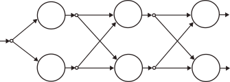
During training, the network accepts a list of pairs of the kind ${(\mathbf{x}^{\mathrm{train}},\mathbf{x}^{\mathrm{train}})}$ .

In the forward pass, ${\mathbf{x}^{\mathrm{train}}}$ is fed to the first layer, each neuron computes its internal variables ${\mathbf{x}^{\mathrm{mid}}, \mathbf{x}^{\mathrm{out}}}$ , passes them on to the next layer and computes its internal derivatives. Finally, the network’s output ${y}$ is produced and the loss ${\mathcal L}$ is computed.

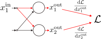
During backpropagation, the loss gradient with respect a layer’s input is first initialized as

$\displaystyle \delta_i := \frac{\mathrm{d} \mathcal L}{\mathrm{d} y_i}, \quad \forall\, i \ \ \ \ \ (18)$

and then updated at each layer in backward fashion, from last to first, via (13):

$\displaystyle \delta_i \leftarrow \sum_{n=1}^N \delta_n \frac{\mathrm{d} x^{\mathrm{out}}_n}{\mathrm{d} x^{\mathrm{in}}_i}, \quad \forall \, i \ \ \ \ \ (19)$

where the term ${\frac{\mathrm{d} x^{\mathrm{out}}_n}{\mathrm{d} x^{\mathrm{in}}_i}}$ is internal to the layer.

At the same time, each layer’s neuron computes the loss gradient with respect to its parameters as in (3)–(4), where the term ${\frac{\mathrm{d} \mathcal L}{\mathrm{d} x^{\mathrm{out}}}}$ corresponds to the back-propagated ${\delta}$ .
Finally, the neuron weights and biases are updated via gradient descent:

$\displaystyle w^i_j \leftarrow w_i^j - \epsilon \, \frac{\mathrm{d} \mathcal L}{\mathrm{d} w^i_j}, \quad \forall\, i,j \ \ \ \ \ (20)$

$\displaystyle b \leftarrow b - \epsilon \, \frac{\mathrm{d} \mathcal L}{\mathrm{d} w^i_j}. \ \ \ \ \ (21)$

Note that, for the sake of simplicity, we simply set ${\epsilon}$ to a constant value here. A notably more efficient choice would be, e.g., Adam optimizer.

from tqdm import tqdm

class FeedForward:
    def __init__(self, layer_len, eps=.0001, seed=None, loss=SquaredLoss, **kwargs):
        self.seed = np.random.randint(int(1e4)) if seed is None else int(seed)
        np.random.seed(self.seed)
        self.layer_len = layer_len
        self.eps = eps
        self.n_layers = len(self.layer_len) - 1
        self.layers = [FullyConnectedLayer(layer_len[ii], layer_len[ii + 1], **kwargs) for ii in range(self.n_layers)]
        self.loss = loss(self.layer_len[-1])
        self.loss_hist = None

    def __call__(self, x):
        # forward pass
        x_in = x
        for ll in range(self.n_layers):
            x_in = self.layers[ll](x_in)
        return x_in

    def backprop(self):
        # gradient backpropagation
        delta = self.layers[-1].update_grad(self.loss.dloss_dy)
        for ll in range(self.n_layers - 1)[::-1]:
            delta = self.layers[ll].update_grad(delta)

    def gradient_descent_par(self):
        # update parameters via gradient descent
        for ll in self.layers:
            for nn in ll.neurons:
                nn.gradient_descent(self.eps)

    def train(self, x_train, y_train, n_iter_max=10000, loss_tol=.1):
        self.loss_hist = np.zeros(n_iter_max)
        x_train, y_train = np.array(x_train), np.array(y_train)
        assert x_train.shape[0] == y_train.shape[0], 'x_train, y_train must contain the same number of samples'
        assert x_train.shape[1] == self.layer_len[0], 'shape of x_train is incompatible with first layer'

        pbar = tqdm(range(n_iter_max))
        for it in pbar:
            loss = 0  # reset loss
            for ii in range(x_train.shape[0]):
                x_out = self(x_train[ii, :])  # forward pass
                loss += self.loss(x_out, y_train[ii, :])  # accumulate loss
                self.backprop()  # backward propagation
                [layer.zero_grad(which=['xin']) for layer in self.layers]  # reset gradient wrt xin to zero
            self.loss_hist[it] = loss
            if (it % 10) == 0:
                pbar.set_postfix_str(f'loss: {loss:.3f}')  #
            if loss < loss_tol:
                pbar.set_postfix_str(f'loss: {loss:.3f}. Convergence has been attained!')
                self.loss_hist = self.loss_hist[: it]
                break
            self.gradient_descent_par()  # update parameters
            [layer.zero_grad(which=['weights', 'bias']) for layer in self.layers]  # reset gradient wrt par to zero

Note that in practice the training data comes in batches, hence the loss and the corresponding gradients are summed across all the batch data. Since gradients are accumulated during the backward pass, they must be reinitialized to zero after each batch.

5. Let’s see from-scratch KAN and MLP in action!

After quite some work, we are finally ready to play with some training data! (see [Jupyter Notebook])

We start with a simple 1D regression problem:

n_iter_train_1d = 500
loss_tol_1d = .05
seed = 476

x_train = np.linspace(-1, 1, 50).reshape(-1, 1)
y_train = .5 * np.sin(4 * x_train) * np.exp(-(x_train+1)) + .5  # damped sinusoid

# KAN training
kan_1d = FeedForward([1, 2, 2, 1],  # layer size
                  eps=.01,  # gradient descent parameter
                  n_weights_per_edge=7,  # n. edge functions
                  neuron_class=NeuronKAN, 
                  x_bounds=[-1, 1],  # input domain bounds
                  get_edge_fun=get_bsplines,  # edge function type (B-splines ot Chebyshev)
                  seed=seed,
                  weights_range=[-1, 1])
kan_1d.train(x_train, 
          y_train, 
          n_iter_max=n_iter_train_1d, 
          loss_tol=loss_tol_1d)

# MLP training
mlp_1d = FeedForward([1, 13, 1],  # layer size
                  eps=.005,  # gradient descend parameter
                  activation=relu,  # activation type (ReLU, tanh or sigmoid)
                  neuron_class=NeuronNN, 
                  seed=seed,
                  weights_range=[-.5, .5])
mlp_1d.train(x_train, 
             y_train, 
             n_iter_max=n_iter_train_1d, 
             loss_tol=loss_tol_1d)

We continue with a slightly more involved 2D regression problem:

def fun2d(X1, X2):
    return X1 * np.power(X2, .5)

X1, X2 = np.meshgrid(np.linspace(0, .8, 8), np.linspace(0, 1, 10))
Y_training = fun2d(X1, X2)

x_train2d = np.concatenate((X1.reshape(-1, 1), X2.reshape(-1, 1)), axis=1)
y_train2d = Y_training.reshape(-1, 1)

We conclude with a classification problem on scikit-learn’s half-moon shaped dataset:

from sklearn import datasets

n_samples = 50
noise = 0.1
x_train_cl, y_train_cl = datasets.make_moons(n_samples=n_samples, noise=noise)

References

[1] Ziming Liu, Yixuan, Sachin Vaidya, Fabian Ruehle, James Halverson, Marin Soljacic, Thomas Y. Hou, Max Tegmark. KAN: Kolmogorov-Arnold networks. arXiv preprint arXiv:2404.19756, 2024 [LINK]

[2] Ziming Liu. YouTube video KAN: Kolmogorov-Arnold Networks [LINK]

[3] Lorenzo Maggi, GitHub repository [LINK]

Posted

May 15, 2024

Deep learning

Lorenzo Maggi

Tags:

KAN, Kolmogorov Arnold Network, MLP, python

Comments

7 responses to “A from-scratch implementation of Kolmogorov-Arnold Networks (KAN)…and MLP”

Melissa Ingle

June 1, 2024

This seems insane (complimentary). Should I spend the next hour trying to get this to work? I can’t get it to work using regular import statements.

LikeLike

Reply
1. Lorenzo Maggi
  
  June 1, 2024
  
  Hi Melissa, thanks for your interest! How can I help? What’s the error?
  
  LikeLike
  
  Reply
Melissa Ingle

June 1, 2024

Oh no worries, I just don’t think I’m smart enough. This explanation is great, and I can follow and really appreciate. When I try to import KAN or do anything with it, I always get the ‘cannot find this module’ error even though I’ve already pip installed it. That’s a me problem though.

LikeLike

Reply
Andrew Polar

July 25, 2024

There are multiple C++ and C# implementations on OpenKAN.org

The training using completely different technique, not the one proposed in MIT article. The performance is 10 to 30 times faster than MLP and even near 10 times faster than C++ implementation of MLP.

MIT article contains reference on this method.

LikeLike

Reply
Gianni Zhang

October 15, 2024

OMG, this is just amazing!!! Thank you very much for sharing, Lorenzo!!!

LikeLike

Reply
Gianni Zhang

October 15, 2024

OMG, this is just amazing! Thank you very much for sharing, Lorenzo!

LikeLike

Reply
1. Lorenzo Maggi
  
  October 15, 2024
  
  Glad you liked it!
  
  LikeLike
  
  Reply

A from-scratch implementation of Kolmogorov-Arnold Networks (KAN)…and MLP

Share this:

Comments

7 responses to “A from-scratch implementation of Kolmogorov-Arnold Networks (KAN)…and MLP”

Leave a comment Cancel reply