Flow matching: Deriving the vector field

Flow matching (FM) is a method that draws ${d}$ -dimensional ( ${d\ge 1}$ ) samples from any (data) distribution ${\pi_Z}$ .

FM` `transforms” noise to data by means of an ordinary differential equation (ODE). The general FM procedure goes like this:

i) Choose an initial (noise) distribution ${\pi_{X_0}}$
ii) Choose the so-called marginal vector field ${u_{t}(\cdot):\mathbb{R}^d \to\mathbb{R}^d}$ for all ${t\in[0,1]}$
iii) Let ${X_t\in \mathbb{R}^d}$ evolve from ${t=0}$ to ${t=1}$ according to the ordinary differential equation (ODE):
$\displaystyle \frac{\mathrm{d}}{\mathrm{d} t} X_t = u_{t}(X_t) \ \ \ \ \ (1)$
$\displaystyle \mathrm{Initial \ condition:} \ X_0\sim \pi_{X_0}.$
iv) The final point ${X_1}$ is distributed as ${\pi_Z}$ .

We will show which choice of the marginal vector field ${u_{t}}$ ensures that item iv) is satisfied, i.e., FM manages to transform noise to data with the correct distribution.

(Notation remarks: Random variables are denoted in capital letters ( ${X,Z}$ ), while their values are denoted in lowercase ( ${x,z}$ ). Generic probability density functions are denoted as ${p(\cdot)}$ .)

1. A first attempt

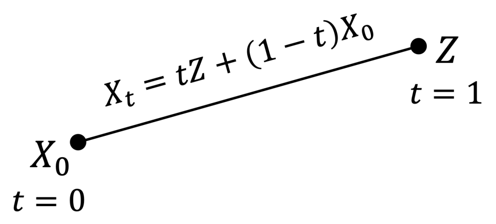
The simplest idea that comes to mind is to transform noise to data via straight lines connecting noise and data points, and hope that there exists an associated ODE that does the same thing. In other words,

1) Define a so-called coupling distribution ${\pi_{X_0,Z}}$ between initial noise ${X_0}$ and data ${Z}$ such that its marginals are the noise and data distributions:
$\displaystyle \int \pi_{(X_0,Z)}(\cdot, z) \, dz = \pi_{X_0}(\cdot) \ \ \ \ \ (2)$ $\displaystyle \int \pi_{(X_0,Z)}(x_0, \cdot) \, dx_0= \pi_{Z}(\cdot) \ \ \ \ \ (3)$
2) Draw random noisy and data pairs ${(X_0,Z)\sim\pi_{(X_0,Z)}}$ .
3) Connect each ${(X_0,Z)}$ with a straight line ${\bar{X}_t := (1-t) X_0 + t Z}$ , defined for all ${t\in[0,1]}$ .
4) For each point ${x\in\mathbb{R}^d}$ and time ${t\in[0,1]}$ , find the (single!) pair of points ${(x_0, z)}$ such that the straight line between them passes through ${x}$ at time ${t}$ , i.e., ${(1-t) x_0 + t z=x}$ .
5) Define ${u_t(x):=z-x_0}$ .

In this way, when the initial point is ${X_0=x_0}$ and ${X_t=x}$ is reached, after an infinitesimal time ${dt}$ , the point ${X_{t+dt}=x + (z-x_0) dt}$ is along the line connecting ${x_0}$ and ${z}$ . Thus, ${X_1=z}$ at the final time ${t=1}$ .

2. When things go well: Data distribution is a Dirac delta

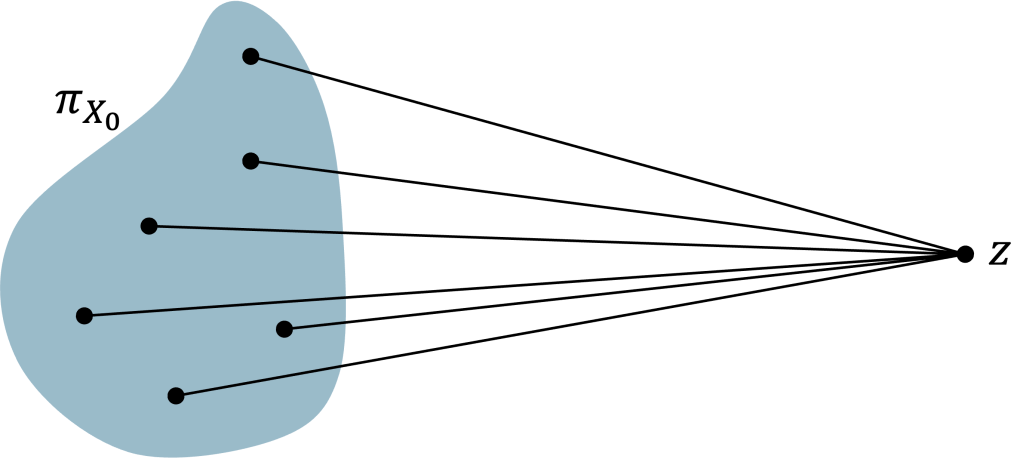
When the data distribution is a Dirac delta, i.e., ${\pi_Z=\delta_z}$ , the pair ${(x_0, z)}$ found in step 4) is unique and the procedure above is well-defined.

In this case, the evolution of ${X_t}$ is governed by the ODE

$\displaystyle \frac{\mathrm{d}}{\mathrm{d} t} X_{t} = \frac{z-X_t}{1-t} := u_{t}(X_t|z) \ \ \ \ \ (4)$

$\displaystyle \mathrm{Initial \ condition:} \ X_0\sim \pi_{X_0}$

where ${u_{t}(\cdot|z)}$ is the so-called conditional vector field.
Clearly, ${X_1=z}$ at the final time ${t=1}$ , i.e., ${\pi_{X_1}\sim \delta_z=\pi_{Z}}$ . So, this simple model manages to transform noise to data with the correct distribution.

(Note: in (4) we rewrote ${u_{t}(X_t|z)=Z-X_0}$ as a function of the current point ${X_t}$ because the vector field should not depend on the initial condition.)

3. When things go wrong and how to fix them

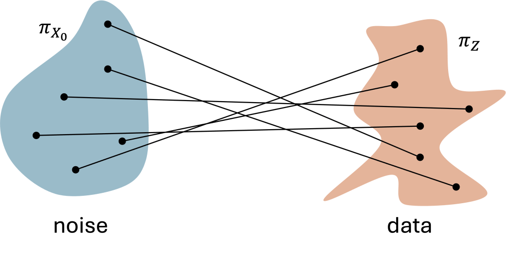
For generic data distributions ${\pi_Z}$ our reasoning has an important flaw at step 4): the line may not be unique! In fact, there may be infinitely many pairs ${(x_0, z)}$ that satisfy the condition ${(1-t) x_0 + t z=x}$ .

How to define ${u_t(x)}$ in this case?

It turns out that the fix is straightforward: it suffices to average the directions ${z-x_0}$ over all the possible pairs ${(x_0, z)}$ that satisfy the condition ${(1-t) x_0 + t z=x}$ . More formally,

$\displaystyle u_t(x) = \mathbb{E}_{(X_0,Z)} \left[ Z-X_0 | \bar{X}_t=x \right] \ \ \ \ \ (5)$

$\displaystyle = \int \!\!\! \int (z-x_0) p_{X_0,Z|\bar{X}_t}(x_0, z | x) \, dx_0 dz.$

Equivalently, we can define ${u_t(x)}$ as the expected value of the conditional vector field ${u_t(x|z)}$ over the data distribution, conditioned on the fact that ${\bar{X}_t=x}$ :

$\displaystyle u_t(x) = \mathbb E_{Z} \left[ u_t(x|Z) | \bar{X}_t=x \right] \ \ \ \ \ (6)$

$\displaystyle = \int u_t(x|z) p_{Z|\bar{X}_t}(z|x) \, dz.$

4. Flow matching reaches its goal

In this final technical section, we prove that FM reaches its goal, i.e., the final point ${X_1}$ of the ODE (1) with vector field ${u_t}$ defined as in (5) or, equivalently, (6) is distributed as the data distribution ${\pi_Z}$ .

Actually, we will prove a slightly more general result: the ODE solution ${X_t}$ is distributed exactly as the random variable ${\bar{X}_t}$ , although their realizations are generated differently. Since ${\bar{X}_1\sim \pi_Z}$ , this achieves our goal.

Our main technical tool is the so-called continuity equation, claiming that if the generic probability density function ${p_t(\cdot)}$ satisfies the following equation:

$\displaystyle \frac{\partial}{\partial t} p_t(x) = -\mathrm{div} \left[ u_t(x) \, p_t(x) \right] \ \ \ \ \ (7)$

then ${X_t}$ , obtained via the ODE (1) with vector field ${u_t}$ , is indeed distributed as ${p_t}$ .

(Note: ${\mathrm{div}}$ is the divergence operator, i.e., ${\mathrm{div}[f(x)] = \sum_{i=1}^d \frac{\partial}{\partial x_i} f_i(x)}$ for any vector field ${f}$ .)

Then, we will show that ${p_{\bar{X}_t}(\cdot)}$ satisfies the continuity equation (7).

$\displaystyle \frac{\partial}{\partial t} p_{\bar{X}_t}(x) = \frac{\partial}{\partial t} \int p_{\bar{X}_t|Z}(x|z) \pi_Z(z) \, dz \ \ \ \ \ (8)$

$\displaystyle \quad = \int \frac{\partial}{\partial t} p_{\bar{X}_t|Z}(x|z) \pi_Z(z) \, dz \ \ \ \ \ (9)$

$\displaystyle \quad = - \int \mathrm{div}\left[ p_{\bar{X}_t|Z}(x|z) u_t(x|z) \right] \pi_Z(z) \, dz \ \ \ \ \ (10)$

$\displaystyle \quad = - \mathrm{div} \left[ \int u_t(x|z) \frac{p_{\bar{X}_t|Z}(x|z) \, \pi_Z(z)}{p_{\bar{X}_t}(x)} \, dz \, p_{\bar{X}_t}(x) \right] \ \ \ \ \ (11)$

$\displaystyle \quad = - \mathrm{div} \left[ u_t(x) p_{\bar{X}_t}(x) \right] \ \ \ \ \ (12)$

where in (10) we applied the continuity equation to the conditional vector field ${u_t(x|z)}$ .

5. Bonus: Equivalence of the two definitions of ${u_t(x)}$

For those who want to check the details, we show here that the definitions (5) and (6) of ${u_t(x)}$ are equivalent.

$\displaystyle \mathbb{E} \left[ Z-X_0 | \bar{X}_t=x \right] = \int \!\!\! \int (z-x_0) \frac{p_{X_0,Z,\bar{X}_t}(x_0, z, x)}{p_{\bar{X}_t}(x)} \, dx_0 dz$