Understanding the adjoint method via backpropagation

In this post, we shed some light on the adjoint state method as used in the famous “Neural ODE” paper [1].

In Section 1, we start by introducing the adjoint state method in its raw form (ODE, loss minimization, adjoint equations), in continuous time (denoted by [C]). If this is already clear to you, then… no need to read the rest of the post! You’re already an adjoint master. Otherwise, please stick with me as we will derive an analogous procedure in discrete time (denoted by [D]) in Section 2, where things are more intuitive.

1. Continuous time: Adjoint method

1.1. ODE formulation

Consider a system that evolves in continuous time and is in state ${x_t\in \mathbb{R}^d}$ at time ${t\in[0,1]}$ . The state evolves according to an ordinary differential equation (ODE):

$\displaystyle \mathrm{[C] \ State \ dynamics:} \quad \frac{\mathrm{d}}{\mathrm{d} t} x_t = f_t(x_t;\theta), \quad \forall \, t\in[0,1] \ \ \ \ \ (1)$

Note that ${f_t: \mathbb R^d \to \mathbb R^d}$ depends on the parameters ${\bar{\theta}\in \mathbb{R}^d}$ , that are typically the weights and biases of a neural network.

A notation remark: ${\theta}$ denotes the decision variable, while ${\bar{\theta}}$ will denote its current value. Similarly, ${x_t}$ is the generic state variable at time ${t}$ , while ${\bar{x}_t}$ shall denote the solution of the ODE (1) at time ${t}$ , given a initial condition ${x_0=x}$ .

1.2. Loss minimization

We want to minimize a penalty ${\mathcal L:=\mathcal L(x_1)}$ by tuning parameters ${\theta}$ appropriately:

$\displaystyle \min_{\theta} \mathcal L \ \ \ \ \ (2)$

Observe that the loss depends on ${\theta}$ through ${x_1}$ , which in turn depends on ${\theta}$ in a complex manner, through the ODE (1).

1.3. Adjoint equations

We now want to compute the gradient of ${\mathcal L}$ with respect to the parameters ${\theta}$ , given the current value ${\bar{\theta}}$ of the parameters and the corresponding solution ${\bar{x}_t}$ of the ODE (1). This will allow us to use gradient descent to minimize (2). To this aim, we first define the adjoint vector ${a_t\in \mathbb{R}^{1\times d}}$ as

$\displaystyle a_t := \frac{\partial \mathcal L}{\partial x_t}, \qquad \forall \, t\in[0,1] \ \ \ \ \ (3)$

which satisfies the following ODE:

$\displaystyle \mathrm{[C] \ Adjoint \ dynamics:} \quad \frac{\mathrm{d}}{\mathrm{d} t} a_t = -a_t \frac{ \partial f_t}{\partial x_t}(\bar{x}_t;\bar{\theta}), \qquad \forall \, t\in[0,1] \ \ \ \ \ (4)$

where ${\frac{\partial f_t}{\partial x_t}(\bar{x}_t;\bar{\theta})\in \mathbb{R}^{d\times d}}$ is to be read as the “Jacobian of ${f_t}$ with respect to state ${x_t}$ evaluated at ${(\bar{x}_t,\bar{\theta})}$ ”. Then, the gradient of ${\mathcal L}$ with respect to the parameters ${\theta}$ , ${\frac{\partial \mathcal L}{\partial \theta}\in \mathbb{R}^{1\times d}}$ , is given by:

$\displaystyle \mathrm{[C] \ Loss \ gradient:} \quad \frac{\partial \mathcal L}{\partial \theta} = \int_0^1 a_t \frac{\partial f_t}{\partial \theta}(\bar{x}_t;\bar{\theta}) dt. \ \ \ \ \ (5)$

1.4. Adjoint method

Fix the current value ${\bar{\theta}}$ of the parameters. To compute ${\frac{\partial \mathcal L}{\partial \theta}}$ , via the adjoint state method, we need to

Solve the ODE (1) forward in time, e.g., with Euler’s method, starting from ${x_0=x}$ to obtain ${\bar{x}_t}$ for all ${t\in[0,1]}$ .
Solve the adjoint equation (4) backward in time, starting from ${a_1 = \frac{\partial \mathcal L}{\partial x_1}}$ , to obtain ${a_t}$ for all ${t\in[0,1]}$ .
Compute the integral (5) to obtain the gradient.

where steps 2 and 3 can be carried out jointly, along a single backward pass.

If little of this is clear to you or you lack the main intuitions, no worries! This post is all about it: we will derive the same procedure in discrete time, where things are more intuitive.

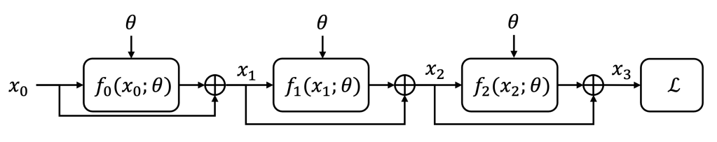
2. Discrete time: Backpropagation

2.1. Discrete-time ODE formulation

To better understand the adjoint method, we construct the discrete-time counterpart of the ODE (1). We will heavily abuse of notation overload, so please bear with me. We start by defining a series of parametric functions ${f_0,\dots,f_{K-1}:\mathbb R^d \to \mathbb R^d}$ such that:

$\displaystyle \mathrm{[D] \ State \ dynamics:} \quad x_{k+1} = x_k + f_{k}(x_{k};\theta), \quad 0\le k<K \ \ \ \ \ (6)$

where ${x_k\in \mathbb R^d}$ is the state at step ${k}$ . Note that this is nothing more that a discretized version of the ODE (1) (the time step is embedded in ${f_k}$ ). In the ML community, equation (6) defines a residual network (ResNet) architecture. The loss ${\mathcal L:=\mathcal L(x_K)}$ depends on the final state ${x_K}$ . Here is a visualization of the discrete-time process with 3 layers ( ${K=3}$ ):

2.2. Loss minimization

As before, our goal is to minimize the loss ${\mathcal L}$ with respect to the parameters ${\theta}$ via gradient descent. To this aim, we need to compute ${\frac{\partial \mathcal L}{\partial \theta}}$ .

2.3. Adjoint equations

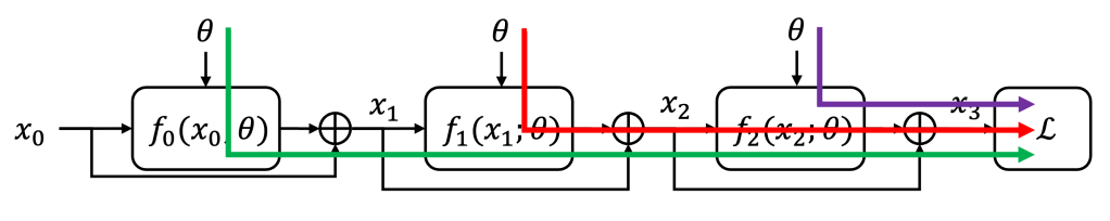
We directly compute the gradient of ${\mathcal L}$ with respect to the parameters ${\theta}$ . We notice that ${\theta}$ appears ${K}$ times in the state evolution, hence any change in ${\theta}$ will propagate towards the loss ${\mathcal L}$ along ${K}$ different paths.

In each path, we can apply the chain rule, as a cascade of two effects: i) the state ${x_k}$ is affected by the parameter ${\theta}$ via the function ${f_{k-1}}$ and varies as ${\frac{\partial f_{k-1}}{\partial \theta}}$ and ii) the loss ${\mathcal L}$ varies as ${\frac{\partial \mathcal L}{\partial x_k}}$ , which is our adjoint variable ${a_k}$ .

We can then sum up the contributions of each one of the ${K}$ paths to obtain

$\displaystyle \mathrm{[D] \ Loss \ gradient:} \quad \frac{\partial \mathcal L}{\partial \theta} = \sum_{k=1}^K a_k \frac{\partial f_{k-1}}{\partial \theta}(\bar{x}_{k-1};\bar{\theta}) \ \ \ \ \ (7)$

where all derivatives are computed at the current value ${\bar{\theta}}$ of the parameters and at the corresponding solution ${\bar{x}}$ of (6) for the initial condition ${x_0=x}$ .

We can recognize that (7) is the discrete-time counterpart of (5), that we report here for convenience:

$\displaystyle \mathrm{[C] \ Loss \ gradient:} \quad \frac{\partial \mathcal L}{\partial \theta} = \int_0^1 a_t \frac{\partial f_t}{\partial \theta}(\bar{x}_t;\bar{\theta}) dt.$

Next we study how the adjoint variables are connected with each other. Recall that ${a_k}$ measures how the loss changes as a function of the state ${x_k}$ . By chain rule, a small change in the state ${x_k}$ impacts the subsequent state ${x_{k+1}}$ via the function ${f_k}$ , which in turns affects the loss:

More formally,

$\displaystyle a_k = a_{k+1} \frac{\partial x_{k+1}}{\partial x_k}(\bar{x}_k;\bar{\theta}). \ \ \ \ \ (8)$

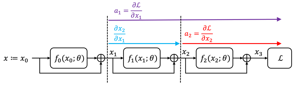
To obtain the analogous of (4), we need to express ${\frac{\partial x_{k+1}}{\partial x_k}}$ in terms of the function ${f_k}$ , via the recursion (6):

$\displaystyle \frac{\partial x_{k+1}}{\partial x_k} = I + \frac{\partial f_{k}}{\partial x_k} \ \ \ \ \ (9)$

where ${I}$ is the identity matrix. Plugging (9) into (8), we obtain for $0\le k < K$ :

$\displaystyle \mathrm{[D] \ Adjoint \ dynamics:} \quad a_{k+1} - a_k = - a_{k+1} \frac{\partial f_{k}}{\partial x_k}(\bar{x}_k;\bar{\theta}) \ \ \ \ (10)$

that is the discrete-time counterpart of the adjoint ODE (4), that we report here for convenience:

$\displaystyle \mathrm{[C] \ Adjoint \ dynamics:} \quad \frac{\mathrm{d}}{\mathrm{d} t} a_t = -a_t \frac{ \partial f_t}{\partial x_t}(\bar{x}_t;\bar{\theta}), \quad \forall \, t\in[0,1].$

2.4. Backpropagation

We now compute the gradient ${\frac{\partial \mathcal L}{\partial \theta}}$ via backpropagation.

First, we need to solve the recursion (6) forward in time starting from the initial condition ${x_0=x}$ and for the current value ${\bar{\theta}}$ of the parameters, to obtain the state succession ${\bar{x}_1, \dots, \bar{x}_K}$ .

Then, in a single backward pass, we solve recursively the adjoint dynamics [D] (10) to obtain ${a_{K-1}, \dots, a_1}$ from the initial seed ${a_K}$ , while accumulating the loss gradient [D] (7). More precisely,

Backpropagation procedure:

0. Set ${\theta = \bar{\theta}}$ and ${x_0 = x}$ .
1. Solve the recursion (6) forward in time to obtain ${\bar{x}_1, \dots, \bar{x}_K}$ .
2. Compute the final adjoint variable ${a_K = \frac{\partial \mathcal L}{\partial x_K}}$ .
3. Initialize the loss gradient ${\frac{\partial \mathcal L}{\partial \theta} = a_K \frac{\partial f_{K-1}}{\partial \theta}(\bar{x}_{K-1};\bar{\theta})}$ .
4. For :
- 4.1. Compute the adjoint ${a_k}$ by solving the adjoint dynamics: ${a_k = a_{k+1} (I + \frac{\partial f_{k}}{\partial x_k}(\bar{x}_k;\bar{\theta}))}$ .
- 4.2. Update the loss gradient ${\frac{\partial \mathcal L}{\partial \theta} \leftarrow \frac{\partial \mathcal L}{\partial \theta} + a_k \frac{\partial f_{k-1}}{\partial \theta}(\bar{x}_{k-1};\bar{\theta})}$ .
5. Return the loss gradient ${\frac{\partial \mathcal L}{\partial \theta}}$ .

Once again, we can recognize that the backpropagation method is the discrete-time counterpart of the adjoint method in Section 1.

You’re now an adjoint master 😉

References

[1] Chen, Ricky TQ, Yulia Rubanova, Jesse Bettencourt, and David K. Duvenaud. “Neural ordinary differential equations.” Advances in neural information processing systems 31 (2018).

Understanding the adjoint method via backpropagation

Share this:

Comments

Leave a comment Cancel reply