Maximum Mean Discrepancy (MMD): The Infinite Moment Matchmaker

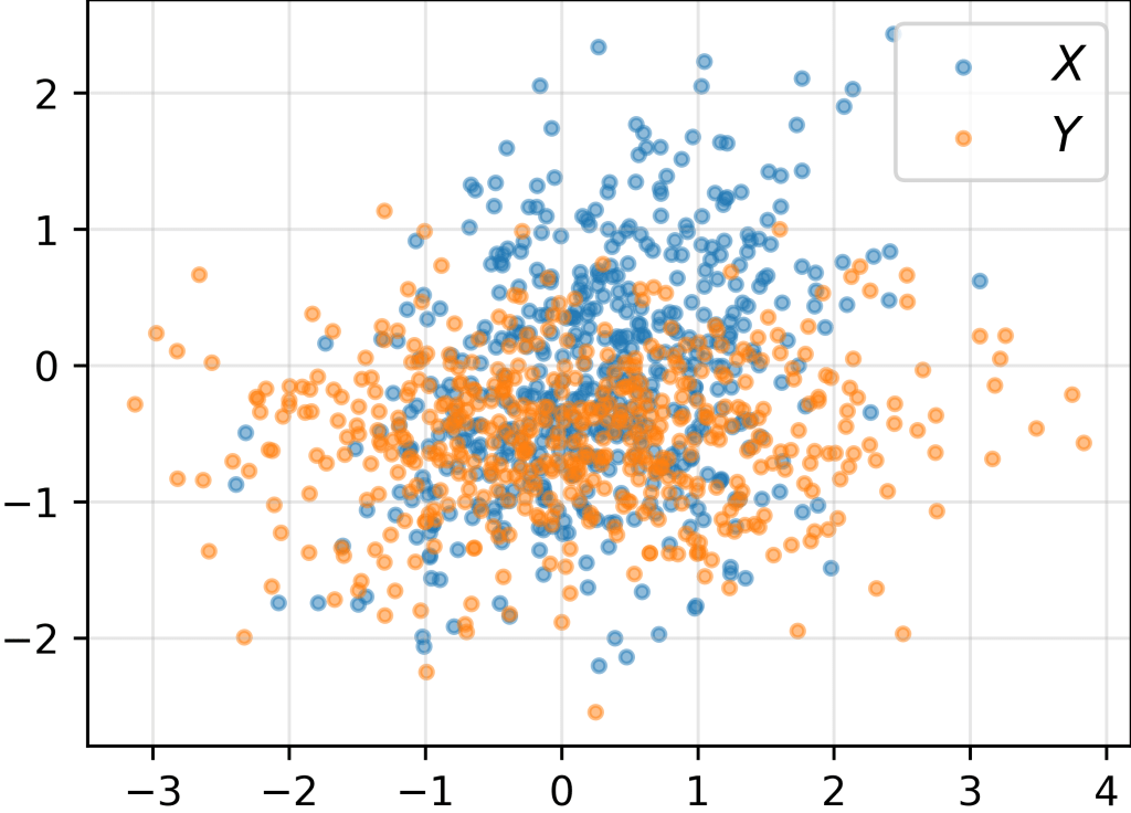
Consider the problem of measuring the discrepancy between the distributions of two sets of samples ${X=\{x_1,\dots,x_n\}}$ and ${Y=\{y_1,\dots,y_m\}}$ .

Amongst various options (KL divergence, Wasserstein distance, etc.), the Maximum Mean Discrepancy (MMD) is a beautifully elegant one, gaining popularity in recent years in the machine learning community.

In this post, instead of defining upfront the MMD in abstract terms (feature space, RKHS, etc.), we first show how to compute it in practice. Afterwards, we will unpack it to derive its formal definition. As a bonus, we will gain insights into MMD’s secret sauce: MMD can be interpreted as a measure of the dissimilarity between all moments of the two distributions.

1. MMD in practice

To compute the empirical MMD between the sets of samples ${X}$ and ${Y}$ , we first need to define the kernel function ${k(q,q')}$ , computing how much two samples ${q}$ and ${q'}$ are similar. A common choice is the Gaussian kernel (also known as Radial Basis Function (RBF) kernel):

$\displaystyle k(q,q') = e^{-\frac{\|q-q'\|^2}{2}}, \quad \forall \, q,q' \in \mathbb{R}^d$

Close-by samples have a high ( ${\approx 1}$ ) kernel value, which tends to 0 as the distance increases. (To keep things simple, we have set the kernel width to 1.)

We then compute the empirical MMD as:

$\displaystyle \widehat{\mathrm{MMD}}^2(X,Y) = \frac{1}{n^2} \sum_{i=1}^n \sum_{j=1}^n k(x_i,x_j) + \frac{1}{m^2} \sum_{i=1}^m \sum_{j=1}^m k(y_i,y_j) \ \ \ \ \ (1)$

$\displaystyle \qquad - \frac{2}{mn} \sum_{i=1}^n \sum_{j=1}^m k(x_i,y_j)$

$\displaystyle \quad = \mathrm{Similarity \ within } \ X + \mathrm{Similarity \ within } \ Y - 2 \times \mathrm{Similarity \ between} \ X \ \mathrm{and} \ Y$

Note that if ${X}$ and ${Y}$ are drawn from the same distribution, the similarity between samples within ${X}$ and ${Y}$ (call it ${s}$ ) is expected to be equal to the similarity between ${X}$ and ${Y}$ . Therefore, the MMD is expected to be close to ${s + s - 2s = 0}$ .

2. MMD in theory

We now want to show that, in its essence, the MMD with RBF kernel computes the dissimilarity between all moments of the two distributions:

$\displaystyle \widehat{\mathrm{MMD}}^2(X,Y) \approx \mathrm{distance}(\mathrm{moments \ of} \ X, \mathrm{moments \ of} \ Y)$

To connect this with the empirical MMD formula above, we need to take two mental steps:

Unpack the RBF kernel
Unpack the empirical MMD formula

2.1. Step 1: Unpack the RBF kernel

We first rewrite the RBF kernel in a more convenient form:

$\displaystyle k(q,q') = e^{-\frac{(q-q')^2}{2}} = e^{-\frac{q^2}{2}} e^{-\frac{q'^2}{2}} e^{q q'}$

(To keep things simple, we have considered unidimensional samples, i.e., ${d=1}$ .)

Then, we develop the cross-product term via Taylor expansion:

$\displaystyle e^{q q'} = \sum_{k=0}^\infty \frac{(q q')^k}{k!}$

$\displaystyle \quad = 1 + q q' + \frac{q^2 q'^2}{2!} + \frac{q^3 q'^3}{3!} + \cdots$

We can then rewrite the kernel as the scalar product of two infinite-dimensional vectors (“features”) ${\varphi(q)}$ and ${\varphi(q')}$ :

$\displaystyle k(q,q') = \langle \varphi(q), \varphi(q') \rangle \ \ \ \ \ (2)$

where:

$\displaystyle \varphi(q) = e^{-\frac{q^2}{2}} \begin{pmatrix} 1, \ q, \ \frac{q^2}{\sqrt{2!}}, \ \frac{q^3}{\sqrt{3!}}, \ \cdots \end{pmatrix}$

$\displaystyle \varphi(q') = e^{-\frac{q'^2}{2}} \begin{pmatrix} 1, \ q', \ \frac{q'^2}{\sqrt{2!}}, \ \frac{q'^3}{\sqrt{3!}}, \ \cdots \end{pmatrix}$

Before we move on to unpack the MMD formula, let’s make a couple of seemingly convoluted but important observations.

Observation 1. Computing the RBF kernel ${k(q,q')}$ can be viewed as a two-step process:

Project the samples ${q}$ and ${q'}$ onto high-dimensional “features” ${\varphi(q)}$ and ${\varphi(q')}$ , respectively.
Compute the scalar product ${\langle \varphi(q), \varphi(q') \rangle}$ between the two features

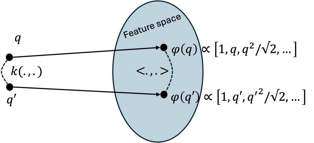
Observation 2. Define the (infinite-dimensional!) vector ${\overline{\varphi}(X)}$ as the average feature of ${X}$ :

$\displaystyle \overline{\varphi}(X) = \frac{1}{n} \sum_{i=1}^n \varphi(x_i)$

Then, ${\overline{\varphi}(X)}$ encodes all empirical moments of the distribution of ${X}$ :

$\displaystyle \overline{\varphi}_k(X) = \frac{1}{n\sqrt{k!}} \sum_{j=1}^n x_i^k, \quad k=0,1,2,\dots \ \ \ \ \ (3)$

As a consequence, MMD compares the variance, the skewness, the kurtosis, etc. of two distributions simultaneously. Let’s show this in detail below.

2.2. Step 2: Unpack the MMD formula

We are now ready to dissect the MMD formula to show that it computes the dissimilarity between all moments of the two distributions.

We plug the definition (2) of the kernel as the inner product of features into the empirical MMD formula (1) to obtain:

$\displaystyle \widehat{\mathrm{MMD}}^2(X,Y) = \frac{1}{n^2} \sum_{i=1}^n \sum_{j=1}^n \langle \varphi(x_i), \varphi(x_j) \rangle + \frac{1}{m^2} \sum_{i=1}^m \sum_{j=1}^m \langle \varphi(y_i), \varphi(y_j) \rangle$

$\displaystyle \qquad - \frac{2}{mn} \sum_{i=1}^n \sum_{j=1}^m \langle \varphi(x_i), \varphi(y_j) \rangle$

By exploiting the linearity property of the inner product, we can rewrite the MMD formula as:

$\displaystyle \widehat{\mathrm{MMD}}^2(X,Y) = \langle \overline{\varphi}(X), \overline{\varphi}(X) \rangle + \langle \overline{\varphi}(Y), \overline{\varphi}(Y) \rangle - 2 \langle \overline{\varphi}(X), \overline{\varphi}(Y) \rangle$

$\displaystyle \qquad = \langle \overline{\varphi}(X) - \overline{\varphi}(Y), \overline{\varphi}(X) - \overline{\varphi}(Y) \rangle$

$\displaystyle \qquad = \|\overline{\varphi}(X) - \overline{\varphi}(Y)\|^2$

Et voilÃ ! The empirical MMD can be rewritten as the squared distance between the mean features of ${X}$ and ${Y}$ , which encode all empirical moments of the distributions, cfr (3).

References

[1] Gretton, A., Borgwardt, K. M., Rasch, M. J., Scholkopf, B., Smola, A. (2012). A kernel two-sample test. The journal of machine learning research, 13(1), 723-773.

Maximum Mean Discrepancy (MMD): The Infinite Moment Matchmaker

Share this:

Comments

Leave a comment Cancel reply