Understanding PPO from first principles

Proximal Policy Optimization (PPO) algorithm is arguably the default choice in modern reinforcement learning (RL) libraries.

In this post we understand how to derive PPO from first principles. First, we brush up our memory on the underlying Markov Decision Process (MDP) model.

1. Preliminaries on Markov Decision Process (MDP)

In an MDP, an agent (say, a robot navigating a maze) interacts with an environment that evolves over time. If at step ${t}$ the agent is in state ${s_t}$ (the robot’s position) and takes action ${a_t}$ (the robot’s velocity vector), then

the agent receives a reward ${r(s_t,a_t)}$ (the robot’s distance from the goal);
the environment transitions to state ${s_{t+1}}$ at the next step ${t+1}$ , with probability ${p(s_{t+1}|s_t,a_t)}$ (the robot’s new position).

Note that the Markov property is assumed: the knowledge of the current state is sufficient to evaluate the transition probability to the next state.

The agent’s behavior is described by policy ${\pi}$ , where ${\pi(a|s)}$ defines the probability of taking action ${a}$ in state ${s}$ . The initial state ${s_0}$ is distributed according to an arbitrary distribution ${\rho_0}$ . The long-term reward is defined as the expected ${\gamma}$ -discounted sum of rewards:

$\displaystyle \eta (\pi) := \mathbb E_{\{s_t,a_t\}_t \sim \pi} \sum_{t\ge 0} \gamma^t r(s_t,a_t) , \quad \gamma\in(0,1). \ \ \ \ \ (1)$

where the notation ${\{s_t,a_t\}_t \sim \pi}$ means that the sequence of states and actions is obtained by following strategy ${\pi}$ .

The agent optimizes its strategy ${\pi}$ to maximize the long-term reward ${\eta}$ :

$\displaystyle \max_{\pi} \eta(\pi). \ \ \ \ \ (2)$

1.1. Advantage function

To improve the performance of a policy, it is important to learn whether a deviation from the base policy brings any benefit. This is formalized by the advantage function. We call ${A_\pi(s,a)}$ the advantage of i) choosing action ${a}$ in state ${s}$ and then following policy ${\pi}$ over ii) adopting ${\pi}$ since state ${s}$ :

$\displaystyle A_\pi(s,a) := r(s,a) + \gamma \sum_{s'} p(s'|s,a) \eta(s',\pi) - \eta(s,\pi). \ \ \ \ \ (3)$

where ${\eta(s,\pi)}$ is the long-term reward when the initial state is ${s}$ . In other words, if ${A_s(a,\pi)>0}$ , then taking action ${a}$ in state ${s}$ is more advantageous than adopting strategy ${\pi}$ .

1.2. Policy parametrization

When the number of states is large, we typically avoid defining the agent’s strategy in each state individually. Instead, it is convenient to define the policy ${\pi}$ as a certain function of (a relatively small number of) parameters ${\theta}$ , that we call ${\pi_{\theta}}$ . Note that ${\theta}$ usually consist of the weights and biases of a neural network.

2. Performance gain ${\Delta}$

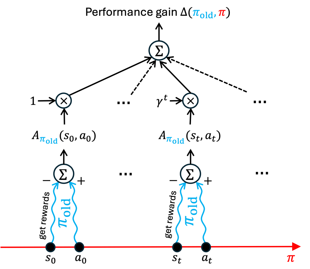
PPO is an algorithm that iteratively improves the performance of an initial policy. It is then useful to evaluate the performance gain ${\Delta(\pi)}$ achieved by a policy ${\pi}$ with respect to a baseline policy ${\pi_{\mathrm{old}}}$ :

$\displaystyle \Delta(\pi_{\mathrm{old}},\pi) := \eta(\pi) - \eta(\pi_{\mathrm{old}}).$

As shown in [1], [2], ${\Delta}$ can be expressed as:

$\displaystyle \Delta(\pi_{\mathrm{old}},\pi) = \mathbb E_{\{s_t,a_t\}_t \sim \pi} \sum_{t\ge 0} \gamma^t A_{\pi_{\mathrm{old}}}(s_t,a_t). \ \ \ \ \ (4)$

The right-hand side of (4) reads as follows:

Follow the new strategy ${\pi}$ and observe a trajectory of actions ${a_0,a_1,\dots}$ and states ${s_1,s_2,\dots}$ . Along this trajectory, evaluate the advantage of taking such actions with respect to the old policy ${\pi^{\mathrm{old}}}$ and sum them up. Finally, take the expectation across all possible trajectories.

Visually:

2.1. A more explicit formula for ${\Delta}$

It is convenient to formulate ${\Delta(\pi_{\mathrm{old}},\pi)}$ more explicitly. We start by rewriting (4) as:

$\displaystyle \Delta(\pi_{\mathrm{old}},\pi) = \sum_{t\ge 0} \gamma^t \sum_{s} \mathbb P (S_t=s|\pi) \sum_{a} \pi(a|s) A_{\pi_{\mathrm{old}}}(s,a).$

We then exchange the sum order:

$\displaystyle \Delta(\pi_{\mathrm{old}},\pi) = \sum_{s\in \mathcal S} \sum_{t\ge 0} \gamma^t \mathbb P (S_t=s|\pi) \sum_{a} \pi(a|s) A_{\pi_{\mathrm{old}}}(s,a)$

and finally write:

$\displaystyle \Delta(\pi_{\mathrm{old}},\pi) = \sum_{s} \rho_\pi(s) \sum_{a} \pi(a|s) A_{\pi_{\mathrm{old}}}(s,a) \ \ \ \ \ (5)$

where ${\rho_\pi(s)}$ is the (discounted) frequency at which MDP visits state ${s}$ over time:

$\displaystyle \rho_\pi(s):=\sum_{t\ge 0} \gamma^t \mathbb{P}(S_t=s|\pi).$

Notice that in expression (5), the effect of policy ${\pi}$ on the state distribution (in the outer sum) is separated from its effect on the actions selected in each state (in the inner sum).

3. How to make ${\Delta}$ positive?

To improve upon our baseline policy ${\pi_{\mathrm{old}}}$ , we want to find a second policy ${\pi}$ such that

$\displaystyle \Delta(\pi_{\mathrm{old}},\pi)\ge 0. \ \ \ \ \ (6)$

Idea 1: Maximizing ${\Delta}$ . This is unfeasible, since this would amount to finding the optimal policy, which is our ultimate goal!

Idea 2: Policy improvement. Let us look back at expression (5). The policy ${\pi}$ influences both the state frequency ${\rho_\pi}$ , in the outer sum, and the action choice, in the inner sum. Unfortunately, the former dependency, between ${\rho}$ and ${\pi}$ , is difficult to characterize. However, notice that the outer terms ${ \rho_\pi(s)}$ are already non-negative. Then, if we can ensure that each inner sum (i.e., the average advantage in each state) is positive, we no longer need to worry about ${\rho_\pi}$ !

In other words, to obtain ${\Delta(\pi_{\mathrm{old}},\pi)\ge 0}$ it suffices that

$\displaystyle \sum_a \pi(a|s) A_{\pi_{\mathrm{old}}}(s,a)\ge 0 \quad \text{in every state } s. \ \ \ \ \ (7)$

Such approach generalizes the classic policy improvement algorithm, that maximizes the advantage function in each state:

$\displaystyle \pi_{\mathrm{PI}}(a^*|s)=1 \quad \text{if} \ a^*=\mathrm{arg\,max}_a A_{\pi^{\mathrm{old}}}(s,a), \quad \forall\, s. \ \ \ \ \ (8)$

However, when the number of states is large, such method presents several issues:

i) Enumerating all states may be infeasible in the first place
ii) The advantage function ${A_{\pi^{\mathrm{old}}}}$ is not known precisely; thus, ${\pi_{\mathrm{PI}}}$ may take wrong decisions resulting in ${\Delta<0}$
ii) When the policy is a parametric function, its degrees of freedom are reduced; hence, optimizing the policy independently in each state becomes impossible.

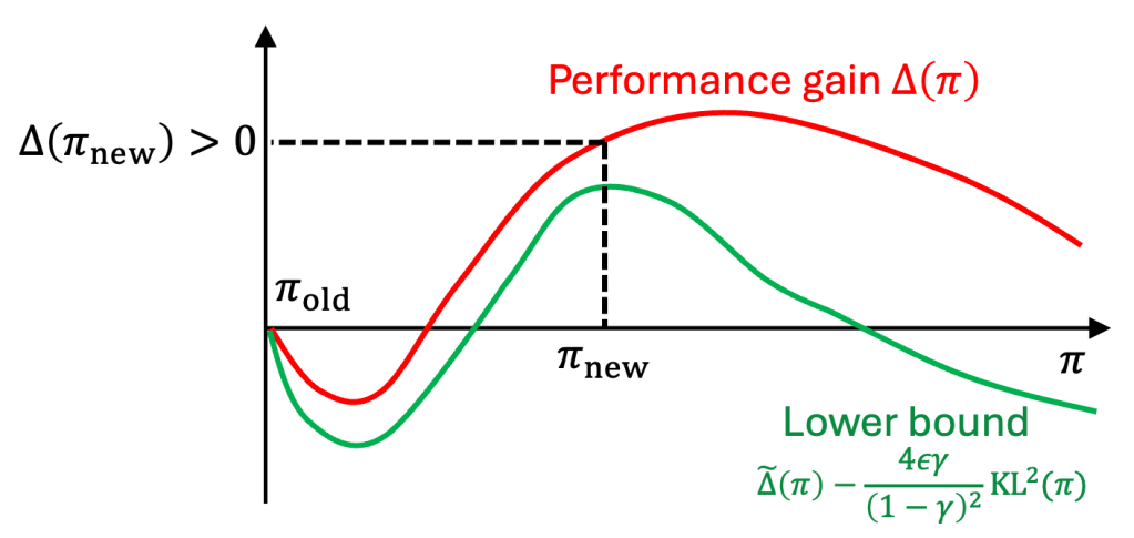
Idea 3: Maximize a lower bound PPO, as well its ancestor TRPO, overcome the limitations above by maximizing a convenient lower bound for ${\Delta}$ . Once the lower bound becomes positive, ${\Delta}$ is guaranteed to be positive as well. Next, we derive such lower bound.

4. A lower bound for the performance gain ${\Delta}$

We derive a lower bound for the performance gain ${\Delta(\pi_{\mathrm{old}},\pi)}$ in three steps.

Step 1: Approximating ${\Delta}$ . As already mentioned, the performance gain ${\Delta(\pi_{\mathrm{old}},\pi)}$ can be decomposed into two components:

(inner sum) the expected action advantage ${\sum_a \pi(a|s) A_{\pi_{\mathrm{old}}}(s,a)}$ in each state ${s}$
(outer sum) the weighted average of the inner terms with respect to the state visitation frequency ${\sum_{s} \rho_\pi(s) \dots}$

It turns out that when a policy ${\pi}$ is “close” to the base policy ${\pi_{\mathrm{old}}}$ , the short-term factor provides the dominant contribution. Thus, we can neglect the dependence of ${\Delta}$ on the state visitation frequency ${\rho_\pi}$ , replacing it with ${\rho_{\pi_{\mathrm{old}}}}$ , induced by the base policy ${\pi_{\mathrm{old}}}$ . This yields the approximate performance gain ${\widetilde{\Delta}(\pi_{\mathrm{old}},\pi)}$ :

$\displaystyle \Delta(\pi_{\mathrm{old}},\pi) \approx \widetilde{\Delta}(\pi_{\mathrm{old}},\pi) \ \ \ \ \ (9)$

$\displaystyle \text{where } \widetilde{\Delta}(\pi_{\mathrm{old}},\pi) := \sum_{s} \rho_{\pi_{\mathrm{old}}}(s) \sum_a \pi(a|s) A_{\pi_{\mathrm{old}}}(s,a). \ \ \ \ \ (10)$

Step 2: Quantify the “closeness” between strategies ${\pi}$ and ${\pi_{\mathrm{old}}}$ . This is done by computing the maximum Kullback–Leibler divergence between the distributions ${\pi_{\mathrm{old}}(\cdot|s),\pi(\cdot,s)}$ across states ${s}$ :

$\displaystyle \mathrm{KL}(\pi_{\mathrm{old}},\pi) = \max_s \sum_a \pi_{\mathrm{old}}(a|s) \log \frac{\pi_{\mathrm{old}}(a|s)}{\pi(a|s)}. \ \ \ \ \ (11)$

Observe that ${\mathrm{KL}(\pi_{\mathrm{old}},\pi)=0}$ means that ${\pi=\pi_{\mathrm{old}}}$ , while higher values of ${\mathrm{KL}}$ indicate larger behavior discrepancies between the two policies in at least one state.

Step 3: Deriving the lower bound for ${\Delta}$ . We can lower bound the performance gain ${\Delta(\pi_{\mathrm{old}},\pi)}$ as the approximate ${\widetilde{\Delta}(\pi_{\mathrm{old}},\pi)}$ minus (a scaled version of) the divergence between the two policies [2]:

$\displaystyle \Delta(\pi_{\mathrm{old}},\pi) \ge \widetilde{\Delta}(\pi_{\mathrm{old}},\pi) - \tfrac{4\epsilon \gamma}{(1-\gamma^2)} \mathrm{KL}^2(\pi_{\mathrm{old}},\pi) \ \ \ \ \ (12)$

where ${\epsilon:= \max_{s,a} |A_{\pi_{\mathrm{old}}}(s,a)|}$ . Next, we discuss why maximizing the lower bound is a good idea, and how to do it.

5. TRPO: Maximize the lower bound

Trust Region Policy Optimization (TRPO) [2], PPO’s direct ancestor, maximizes the performance gain lower bound (12):

$\displaystyle \pi_{\mathrm{TRPO}} = \mathrm{arg\, max}_{\pi} \widetilde{\Delta}(\pi_{\mathrm{old}},\pi) - \tfrac{4\epsilon \gamma}{(1-\gamma^2)} \mathrm{KL}^2(\pi_{\mathrm{old}},\pi). \ \ \ \ \ (13)$

In this case, we strive to jointly

Select advantageous actions to increase the approximate gain ${\widetilde{\Delta}(\pi_{\mathrm{old}},\pi)}$
Remain close to the base policy ${\pi_{\mathrm{old}}}$ to reduce the KL divergence.

Observe that, as a side-product, the latter point is of practical importance to ensure stability.

As promised, ${\Delta(\pi_{\mathrm{old}},\pi_{\mathrm{TRPO}})\ge 0}$ . This stems from its lower bound being nonnegative, as illustrated below.

5.1. Towards practice (1): Turn penalty into constraint

In practice, the coefficient penalizing the ${\mathrm{KL}}$ divergence in TRPO forces tiny policy update and is hard to tune it. A better option is to replace the penalty on ${\mathrm{KL}}$ with a hard constraint, in a way reminiscent of Lagrangian theory. Thus, we maximize the approximate gain while remaining “close” to ${\pi_{\mathrm{old}}}$ :

$\displaystyle \pi_{\text{C-}\mathrm{TRPO}} = \mathrm{arg\,max}_{\pi} \widetilde{\Delta}(\pi_{\mathrm{old}},\pi) \ \ \ \ \ (14)$

$\displaystyle \text{s.t.} \ \mathrm{KL}(\pi_{\mathrm{old}},\pi) \le \delta.$

5.2. Towards practice (2): Estimating ${\widetilde{\Delta}}$ via sample averages

Computing the analytical expression of ${\widetilde{\Delta}(\pi_{\mathrm{old}},\pi)}$ (10) is challenging due to the presence of the state frequency ${\rho_{\pi_{\mathrm{old}}}}$ .

Estimating ${\widetilde{\Delta}(\pi_{\mathrm{old}},\pi)}$ turns out to be easier. In fact, one can

Express it as an expectation with respect to the base policy ${\pi_{\mathrm{old}}}$ ;
Compute empirical averages across multiple trajectories obtained by following ${\pi_{\mathrm{old}}}$ .

In detail, we first multiply and divide each term of the inner sum of expression (10) by ${\pi_{\mathrm{old}}(a|s)}$ (assuming it is positive).

$\displaystyle \widetilde{\Delta}(\pi_{\mathrm{old}},\pi) = \sum_{s} \rho_{\pi_{\mathrm{old}}}(s) \sum_a \pi_{\mathrm{old}}(a|s) \pi(a|s) \frac{A_{\pi_{\mathrm{old}}}(s,a)}{\pi_{\mathrm{old}}(a|s)} .$

Then, we can estimate ${\Delta(\pi_{\mathrm{old}},\pi)}$ as the empirical average ${\widehat{\mathbb E}}$ across trajectory roll-outs ${a_0,s_1,a_1,\dots}$ generated by the old strategy ${\pi_{\mathrm{old}}}$ :

$\displaystyle \widetilde{\Delta}(\pi_{\mathrm{old}},\pi) \approx \widehat{\mathbb{E}}_{\{s_t,a_t\}_t \sim \pi_{\mathrm{old}}} \sum_{t\ge 0} \gamma^t \pi(a_t|s_t) \frac{A_{\pi_{\mathrm{old}}}(s_t,a_t)}{\pi_{\mathrm{old}}(a_t|s_t)}. \ \ \ \ \ (15)$

Visually:

5.3. Towards practice (3): Estimating the advantage function

In this post we do not discuss how to estimate the advantage function. For this, the reader is encouraged to consult the excellent reference [4].

5.4. Addressing the issues of policy improvement

As promised, TRPO solves (or at least, mitigates) the issues with policy improvement (PI):

i) Unlike PI, TRPO does not need to enumerate all states;
ii) TRPO is more robust to uncertainties in the advantage function than PI, since TRPO maximizes an aggregate advantage function rather than each individual advantage term ${A(s,\cdot)}$ ;
iii) For the same reason, TRPO is more suitable than PI for parametric policies, for which actions cannot be optimized independently in each state.

5.5. All that glitters is not (yet) gold

Finding the constrained TRPO policy ${\pi_{\text{C-}\mathrm{TRPO}}}$ by solving the optimization problem (14) is still hard, due to the constraint on the KL divergence. This is where PPO comes to the rescue, as we will see next.

6. Proximal Policy Optimization (PPO)

PPO gets away with the hard-to-handle TRPO’s constraint on the KL divergence by re-incorporating it in the objective function in a friendly way, i.e., solvable by gradient descent. To understand how, we follow 4 steps.

Step 1. Let us first recall informally TRPO’s goal:

Maximize the approximate performance gain ${\widetilde{\Delta}(\pi_{\mathrm{old}},\pi)}$ while maintaining the new policy ${\pi}$ close to the old policy ${\pi_{\mathrm{old}}}$ .

Step 2. What goes wrong when we omit the constraint on ${\pi}$ being close to ${\pi_{\mathrm{old}}}$ ? In this case, we would simply maximize ${\widetilde{\Delta}}$ :

$\displaystyle \max_\pi \widetilde{\Delta}(\pi_{\mathrm{old}},\pi) := \widehat{\mathbb{E}}_{\{s_t,a_t\}_t \sim \pi_{\mathrm{old}}} \sum_{t\ge 0} \gamma^t \pi(a_t|s_t) \frac{A_{\pi_{\mathrm{old}}}(s_t,a_t)}{\pi_{\mathrm{old}}(a_t|s_t)}.$

The optimal policy would tend to assign high probability to actions with a large ratio “advantage” to “probability of being chosen by the old policy”:

$\displaystyle \text{Select the action } a \text{ with the highest} \ \tfrac{A_{\pi_{\mathrm{old}}}(s,a)}{\pi_{\mathrm{old}}(a|s)}, \ \forall \, s. \ \ \ \ \ (16)$

Visually:

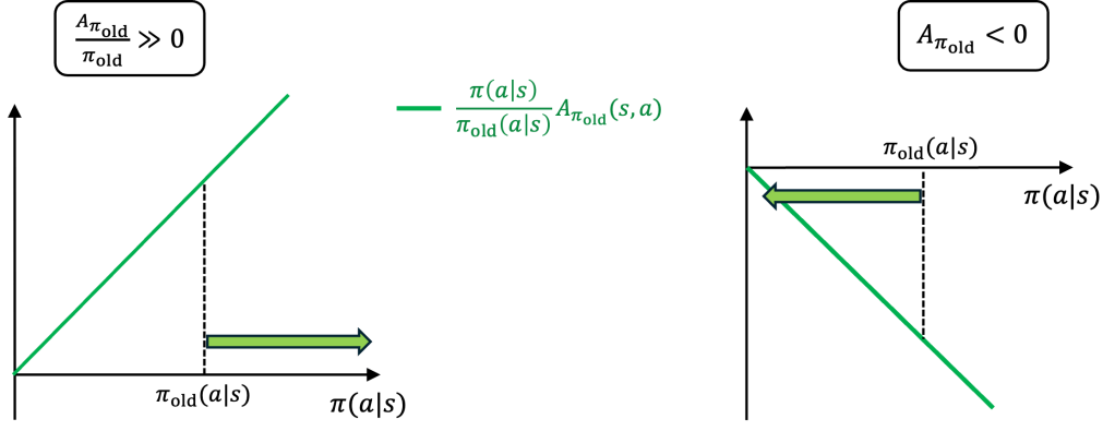
Thus, actions that were chosen very infrequently under ${\pi_{\mathrm{old}}}$ but have even a slightly positive advantage would be heavily favored by the new policy. This is risky: the less frequently an action is selected, the less accurate its advantage estimate. Therefore, the risk of overcommitting to suboptimal actions is high.

On the other hand, actions with an even slightly negative advantage would be completely ruled out. Again, this is not wise, due to the advantage estimation inaccuracies.

Step 3. PPO prevents the issues above by artificially limiting the reward for choosing policies that deviate too far from the old policy ${\pi_{\mathrm{old}}}$ . In this way, the new policy naturally remains in a close neighborhood of ${\pi_{\mathrm{old}}}$ .

In details, PPO maximizes a new objective function

$\displaystyle \max_{\pi} \, \widehat{\mathbb{E}}_{\{s_t,a_t\}_t \sim \pi_{\mathrm{old}}} \sum_{t\ge 0} \gamma^t L^{\mathrm{clip}}_\pi(s_t, a_t). \ \ \ \ \ (17)$

where the individual terms ${L^{\mathrm{clip}}}$ are defined as

$\displaystyle L^{\mathrm{clip}}_\pi(s_t, a_t) := \min \left\{ \tfrac{\pi(a_t|s_t)}{\pi_{\mathrm{old}}(a_t|s_t)}A_{\pi_{\mathrm{old}}}(s_t,a_t), \mathrm{clip}\left( \tfrac{\pi(a_t|s_t)}{\pi_{\mathrm{old}}(a_t|s_t)}, 1-\epsilon,1+\epsilon \right) A_{\pi_{\mathrm{old}}}(s_t,a_t) \right\} \ \ \ \ \ (18)$

The equation above is best understood via an illustration:

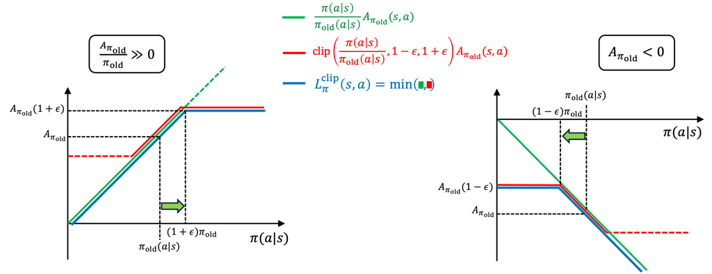
This shows that even when action ${a}$ exhibits a large ratio ${\frac{A_{\pi_{\mathrm{old}}}(s,a)}{\pi_{\mathrm{old}}(a|s)}}$ , PPO has no incentive to place all its weight on ${a}$ , since the associated reward plateaus. Instead, it will increase its probability of being selected by a small amount with respect to ${\pi_{\mathrm{old}}}$ , on the order of ${1+\epsilon}$ . Similarly, when an action has a negative advantage, PPO will benefit only from slightly decreasing its probability of being chosen.

Step 4. PPO can now be solved via gradient descent. The policy ${\pi}$ to be optimized is chosen to be a parametric one, ${\pi_{\theta}}$ , where ${\theta}$ is the set of parameters. Importantly, ${\pi_{\theta}(a|s)}$ must be differentiable with respect to ${\theta}$ , for every state ${as}$ and action ${a}$ . This ensures that the PPO’s objective function is differentiable, enabling the parameters ${\theta}$ to be optimized using gradient-based techniques, which are well understood and efficient.

6.1. PPO’s main steps

To sum up, here are the main steps of PPO algorithm:

a) Start from an arbitrary randomized policy ${\pi_{\mathrm{old}}}$
b) Repeat until convergence:
- 1) Run policy ${\pi_{\mathrm{old}}}$ and collect trajectories ${s_0, a_1,s_1,a_1,\dots}$
- 2) Estimate the advantage function ${A_{\pi_{\mathrm{old}}}(s_t,a_t)}$ , for all steps ${t\ge 0}$
- 3) Solve via gradient-based methods: $\displaystyle \theta^* = \mathrm{arg\,max}_{\theta} \, \widehat{\mathbb{E}}_{\{s_t,a_t\}_t \sim \pi_{\mathrm{old}}} \left[ \sum_{t\ge 0} \gamma^t L^{\mathrm{clip}}_{\pi_{\theta}}(s_t, a_t) \right]$
- 4) Replace ${\pi_{\mathrm{old}} \leftarrow \pi_{\theta^*}}$

References

[1] Kakade, S., Langford, J. (2002, July). Approximately optimal approximate reinforcement learning. In Proceedings of the nineteenth international conference on machine learning (pp. 267-274).

[2] Schulman, J., Levine, S., Abbeel, P., Jordan, M., Moritz, P. (2015, June). Trust region policy optimization. In International conference on machine learning (pp. 1889-1897). PMLR.

[3] Schulman, J., Wolski, F., Dhariwal, P., Radford, A., Klimov, O. (2017). Proximal policy optimization algorithms. arXiv preprint arXiv:1707.06347.

[4] Schulman, J., Moritz, P., Levine, S., Jordan, M., Abbeel, P. (2015). High-Dimensional Continuous Control Using Generalized Advantage Estimation arXiv:1506.02438.

Comments

2 responses to “Understanding PPO from first principles”

Emilien

November 20, 2025

Hey, I think there is a small typo in the last equation (PPO objective, Eq. 18). The A_{pi_old}(s,a) is missing in the left side of the minimum (correctly referenced in the plot bellow as the green curve).
Cool BP, cheers.

LikeLike

1. Lorenzo Maggi
  
  November 20, 2025
  
  Thanks Emilien, good catch 🙂 Just fixed
  
  LikeLike

Understanding PPO from first principles

Share this:

Comments

2 responses to “Understanding PPO from first principles”

Leave a comment Cancel reply