Lagrangian multipliers, normal cones and KKT optimality conditions

We consider constrained optimization problems of the kind:

$\displaystyle \mathbf{x}^* \in \mathrm{argmax}_{\mathbf{x} \in \mathcal F} f(\mathbf{x}) \ \ \ \ \ (1)$

where the feasibility region ${\mathcal F}$ is a polytope, i.e., ${\mathcal F}$ is the set of ${\mathbf{x}}$ such that:

$\displaystyle \begin{array}{ll} \mathbf{Ax} \le \mathbf{b} \\ \mathbf{Cx} = \mathbf{d} \end{array}$

where ${\mathbf{A,C}}$ are real matrices of size ${M\times N}$ and ${L\times N}$ , respectively, and ${\mathbf{b},\mathbf{d}}$ are column vectors. Equivalently, we can rewrite (1) as:

$\displaystyle \mathbf{x}^* \in \mathrm{argmax}_{\mathbf{x}} f(\mathbf{x}) \ \ \ \ \ (2)$

$\displaystyle \mathrm{s.t.} \ \mathbf{a}^{(i)} \cdot \mathbf{x} \le b_i, \quad \forall \, i=1,\dots,M$

$\displaystyle \quad \mathbf{c}^{(\ell)} \cdot \mathbf{x} = d_{\ell}, \quad \forall \, \ell=1,\dots,L$

where ${\mathbf{a}^{(i)},\mathbf{c}^{(i)}}$ are the ${i}$ -th row of ${\mathbf{A}}$ and ${\mathbf{C}}$ , respectively, and ${\cdot}$ denotes the scalar product.

In this post we will study necessary conditions that function ${f}$ must satisfy at any optimal point ${\mathbf{x}^*}$ . These are the so-called Karush-Kuhn-Tucker (KKT) conditions [1,2], which generalize the classic Lagrangian conditions that are valid under equality constraints only.

1. Basic principle and three open questions

In simple words, KKT conditions state that in a neighborhood of any optimal ${\mathbf{x}^*}$ within the feasible region, the function ${f}$ must not increase. This requirement is intuitive but leaves us with some open questions like:

What a (feasible) neighborhood looks like?
How to know whether ${f}$ does not increase within the neighborhood?
How to restate the optimality condition in a form that is actually computable, rather than merely as an abstract definition?

Next we will answer all three questions using geometric insights. Finally, we will also provide an example where KKT conditions actually help us solve the optimization problem.

2. Non-increasing property

Let us place ourselves at the optimum ${\mathbf{x}^*}$ . We look towards all directions emanating from ${\mathbf{x}^*}$ and we select only those that, if followed even for a tiny bit, allow ourselves to stay within the feasible region. We denote such feasible directions as ${\mathcal F_{\mathbf{x}^*}}$ and will characterize them in the next section.

Along the feasible direction ${\mathbf{v}\in \mathcal{F}_{\mathbf{x}^*}}$ , function ${f}$ must not increase, at least locally. In other words, its directional derivative must be null or negative. We recall that such derivative equals the scalar product between the gradient ${\nabla f(\mathbf{x}^*)=[\frac{df}{dx_1}(\mathbf{x}^*),\dots,\frac{df}{dx_N}(\mathbf{x}^*)]}$ and ${\mathbf{v}}$ . Thus, the optimality condition can be written as:

$\displaystyle \nabla f(\mathbf{x}^*) \cdot \mathbf{v} \le 0, \quad \forall \, \mathbf{v} \in \mathcal{F}_{\mathbf{x}^*}. \ \ \ \ \ (3)$

Condition (3) is a valid necessary optimality condition, although still quite primitive, since ${\mathcal{F}_{\mathbf{x}^*}}$ is not defined (yet). However, an important—although not surprising—conclusion stems from it. If ${\mathbf{x}^*}$ lies in the interior of the feasibility region ${\mathcal F}$ , then we can safely travel along any direction without falling outside ${\mathcal F}$ . Then, ${\mathcal{F}_{\mathbf{x}^*}}$ coincides with the whole set ${\mathbb{R}^N}$ , hence the gradient must be necessarily null for (3) to hold:

$\displaystyle \nabla f(\mathbf{x}^*)=0 \quad \mathrm{if} \ \mathbf{x}^* \in \text{ interior of } \mathcal F$

which is the classic first-order optimality condition for unconstrained optimization.

3. Feasible directions ${\mathcal{F}_{\mathbf{x}^*}}$

We next refine the optimality condition (3) by characterizing the set of feasible directions ${\mathcal{F}_{\mathbf{x}^*}}$ , being the directions along which we can depart from ${\mathbf{x}^*}$ while staying within the feasibility region, even for a small distance.

As it turns out, ${\mathcal{F}_{\mathbf{x}^*}}$ can be simply defined as the set of vectors ${\mathbf{v}}$ translating ${\mathbf{x}^*}$ to any other feasible point ${\mathbf{x}}$ :

$\displaystyle \mathcal{F}_{\mathbf{x}^*} = \left\{ \mathbf{v}=\mathbf{x}-\mathbf{x}^*, \ \forall\, \mathbf{x}\in\mathcal{F} \right\}. \ \ \ \ \ (4)$

This stems from the convexity property of the feasibility region ${\mathcal F}$ : if ${\mathbf{x}}$ is feasible, then any point between ${\mathbf{x}^*}$ and ${\mathbf{x}}$ is feasible. The same does not hold if ${\mathcal F}$ were not convex, as illustrated below.

We can now make the optimality condition (3) more explicit by rewriting it as:

$\displaystyle \nabla f(\mathbf{x}^*) \cdot (\mathbf{x} - \mathbf{x}^*) \le 0, \quad \forall\, \mathbf{x} \in \mathcal F. \ \ \ \ \ (5)$

Although we’ve made headway, there is still something unsatisfying about condition (5): validating the relationship across all feasible points feels like too daunting of a task. We will take care of this in the next section.

4. KKT conditions via normal cones

Condition (5) states that, in order for ${\mathbf{x}^*}$ to be optimal, the gradient ${\nabla f(\mathbf{x}^*)}$ must be anti-aligned with all feasible directions departing from ${\mathbf{x}^*}$ , since its scalar product with each of them is non-positive. More formally, we say that ${\nabla f(\mathbf{x}^*)}$ belongs to the normal cone of ${\mathcal F}$ at ${\mathbf{x}^*}$ , referred to as ${\mathcal N_{\mathbf{x}^*}}$ :

$\displaystyle \nabla f(\mathbf{x}^*) \in \mathcal N_{\mathbf{x}^*} \ \ \ \ \ (6)$

$\displaystyle \text{where } \mathcal N_{\mathbf{x}^*} = \left\{ \mathbf{x}': \ \mathbf{x}' \cdot (\mathbf{x}-\mathbf{x}^*) \le 0, \ \forall\, \mathbf{x}\in\mathcal F \right\}.$

In the hope of further refining condition (5), we are then interested in characterizing ${\mathcal N_{\mathbf{x}^*}}$ in explicit form.

We build up to its general definition via examples of increasing complexity.

(Temporarily) discard equality constraints ${\mathbf{Cx}= \mathbf{d}}$ . In the next few examples we will then consider only constraints of the kind ${\mathbf{Ax}\le \mathbf{b}}$ . We will later realize that this simplification is actually without loss of generality.

The optimum is inside ${\mathcal F}$ . If the ${\mathbf{x}^*}$ is in the interior of ${\mathcal F}$ then the normal cone ${\mathcal N_{\mathbf{x}^*}=0}$ , as we already discussed:

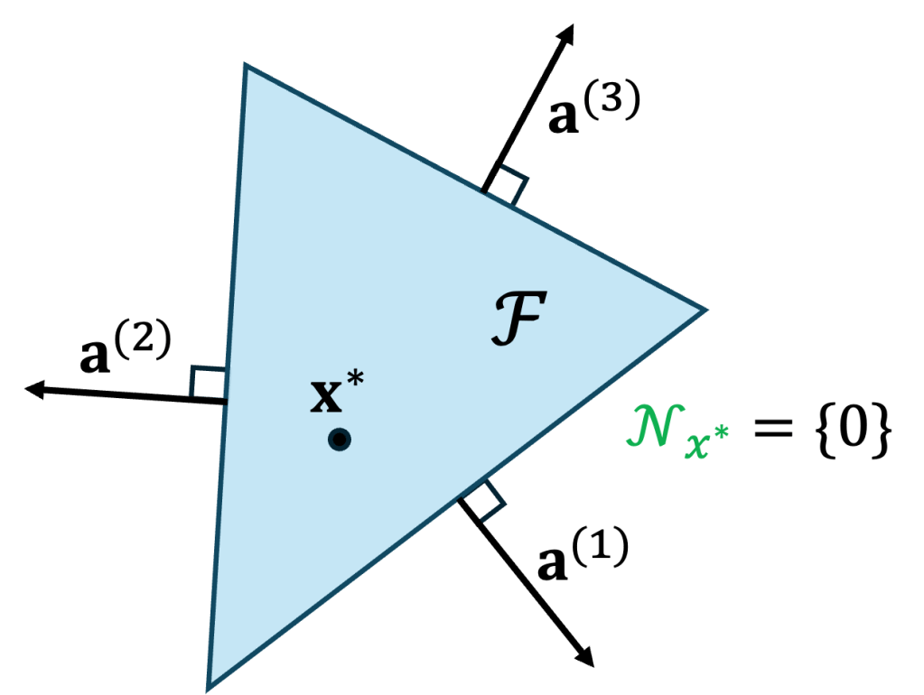
One constraint is tight. Next, we suppose that ${\mathbf{x}^*}$ satisfies exactly one constraint, say the first one, with equality, while the remaining are satisfied with strict inequality. In this case, ${\mathbf{x}^*}$ lies on an edge of ${\mathcal F}$ and the normal cone ${\mathcal N_{\mathbf{x}^*}}$ coincides with the half line spanning from ${\mathbf{a}^{(1)}}$ :

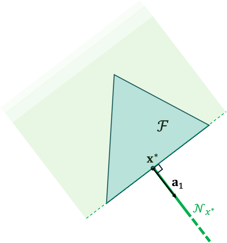
Observe that the green shaded region denotes the set of vectors that are anti-aligned with ${\mathbf{a}^{(1)}}$ , i.e., their scalar product is non-positive. Note that it must contain the whole feasibility set ${\mathcal F}$ for ${\mathbf{a}^{(1)}}$ to belong to ${\mathcal N_{\mathbf{x}^*}}$ .

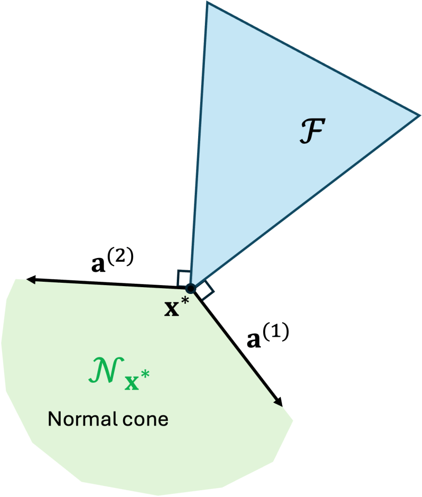
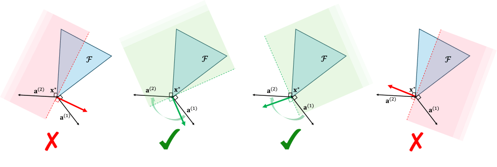
Two constraints are tight. When two constraints are tight—say the first two—instead of just one, the feasibility region ${\mathcal F}$ shrinks. Hence, we expect that i) the normal cone ${\mathcal N_{\mathbf{x}^*}}$ enlarges and ii) ${\mathbf{a}^{(1)},\mathbf{a}^{(2)}}$ still belong to ${\mathcal N_{\mathbf{x}^*}}$ . Pushing the reasoning further, the visual argument below should convince us that iii) ${\mathcal N_{\mathbf{x}^*}}$ coincides with all vectors lying in between ${\mathbf{a}^{(1)}}$ and ${\mathbf{a}^{(2)}}$ :

More formally, ${\mathcal N_{\mathbf{x}^*}}$ is the cone spanned by ${\mathbf{a}^{(1)}}$ and ${\mathbf{a}^{(2)}}$ :

$\displaystyle \mathcal N_{\mathbf{x}^*} = \left\{ \mathbf{x}=\lambda_1 \mathbf{a}^{(1)} + \lambda_2 \mathbf{a}^{(1)}, \ \forall\, \lambda_1,\lambda_2\ge 0 \right\} \ \ \ \ \ (7)$

where ${\lambda_1,\lambda_2}$ are the so-called Lagrangian multipliers.

Multiple constraints are tight. The same intuitions we just gained with two tight constraints also apply when dealing with multiple tight constraints. To give a final polish to our expression of ${\mathcal N_{\mathbf{x}^*}}$ and make explicit that only the ${\mathbf{a}}$ ‘s associated with the tight constraints contribute to forming the normal cone, we can write

$\displaystyle \mathcal N_{\mathbf{x}^*} = \left\{ \mathbf{x}=\sum_{i=1}^M \lambda_i \mathbf{a}^{(i)}, \ \forall\, \lambda_i\ge 0, \ i=1,\dots,M \right\} \ \ \ \ \ (8)$

$\displaystyle \lambda_i \left( \mathbf{a}^{(i)}\cdot \mathbf{x}^*-b_i \right) = 0, \quad \forall\, i=1,\dots,M. \ \ \ \ \ (9)$

where (9) is the complementary slackness condition, claiming that

if the ${i}$ -th constraint is loose, i.e., ${\mathbf{a}^{(i)}\cdot \mathbf{x}^* < b_i}$ , then ${\lambda_i=0}$ , thus ${\mathbf{a}^{(i)}}$ does not contribute to ${\mathcal N_{\mathbf{x}^*}}$ ;
if the ${i}$ -th constraint is tight, i.e., ${\mathbf{a}^{(i)}\cdot \mathbf{x}^* = b_i}$ , then ${\lambda_i\ge 0}$ , thus ${\mathbf{a}^{(i)}}$ can intervene in forming ${\mathcal N_{\mathbf{x}^*}}$ .

Bringing back equality constraint. We now what we have learnt so far to the initial case with inequality constraints ${\mathbf{Ax}\le \mathbf{b}}$ and equality constraints ${\mathbf{Cx}=\mathbf{d}}$ .

Let us start simple: in the presence of just one equality constraint ${\mathbf{c}\cdot \mathbf{x}=d}$ , the normal cone at ${\mathbf{x}^*}$ is the whole line perpendicular to ${\mathcal F}$ , hence parallel to ${\mathbf{c}}$ , passing through ${\mathbf{x}^*}$ :

Observe that unlike the inequality case, where multipliers are nonegative, the normal cone is formed by scaling ${\mathbf{c}}$ by a multiplier that can be either positive or negative.

To make this statement more formal, we first rewrite every equality constraint ${\mathbf{c}^{(\ell)}\cdot \mathbf{x}=d_{\ell}}$ as two inequalities:

$\displaystyle \mathbf{c}^{(\ell)}\cdot \mathbf{x} \le d_{\ell}$

$\displaystyle -\mathbf{c}^{(\ell)}\cdot \mathbf{x} \le -d_{\ell}$

Then, we assign nonnegative Lagrangian multipliers ${\mu_{\ell}',\mu_{\ell}''\ge 0}$ to the two previous inequalities, for all ${\ell}$ , and integrate those in our previous definition of normal cone in (8) to obtain:

$\displaystyle \mathcal N_{\mathbf{x}^*} = \left\{ \mathbf{x}=\sum_{i=1}^M \lambda_i \mathbf{a}^{(i)} + \sum_{\ell=1}^L (\mu_{\ell}'-\mu_{\ell}'') \mathbf{c}^{(\ell)}, \ \forall\, \lambda_i,\mu'_{\ell},\mu''_{\ell}\ge 0, \forall\, i,\ell \right\} \ \ \ \ \ (10)$

It is convenient to assign just one multiplier ${\mu_{\ell}=\mu_{\ell'}-\mu_{\ell''}}$ to the ${\ell}$ -th equality constraint; note that ${\mu_{\ell}}$ can be either positive or negative, as previously predicted!

We also observe that the complementary slackness condition (9) still holds the same, since equality constraitns are tight by definition.

Putting all together: KKT conditions. After quite some work, we are finally ready to provide the polished version of KKT optimality conditions.

If ${\mathbf{x}^*}$ is an optimal solution to the optimization problem ${\max_{\mathbf{Ax}\le \mathbf{b}, \mathbf{Cx}=\mathbf{d}} f(\mathbf{x})}$ , then there must exist ${\{\lambda_i\ge 0,\mu_{\ell}\}}$ such that:

$\displaystyle \nabla f(\mathbf{x}^*) = \sum_{i=1}^M \lambda_i \mathbf{a}^{(i)} + \sum_{\ell=1}^L \mu_{\ell} \mathbf{c}^{(\ell)} \ \ \ \ \ (11)$

$\displaystyle \lambda_i \left( \mathbf{a}^{(i)}\cdot \mathbf{x}^*-b_i \right) = 0, \quad \forall\, i=1,\dots,M.$

5. A formal proof

For those who want to go deeper, below we prove that the normal cone at point ${\mathbf{x}^*}$ coincides with the cone spanned by the ${\mathbf{a}}$ ‘s corresponding to the constraints which are tight at ${\mathbf{x}^*}$ , as claimed by expressions (8)–(9).

Theorem 1 Let ${\mathcal{F}=\{\mathbf{x}: \ \mathbf{a}^{(i)} \cdot \mathbf{x} \le b_i, \ \forall \, i=1,\dots,M\}}$ be the feasibility region with inequalities only and call ${\mathcal I_{\mathbf{x}^*}=\{ i: \ \mathbf{a}^{(i)} \cdot \mathbf{x}^* = b_i \}}$ the set of constraints being tight at point ${\mathbf{x}^*}$ . Define ${\mathcal Y_{\mathbf{x}^*}=\{ \mathbf{x}=\sum_{i \in \mathcal I(\mathbf{x}^*)} \lambda_i \mathbf{a}^{(i)}, \ \forall\, \lambda_i\ge 0\}}$ the cone spanned by ${\mathbf{a}}$ ‘s corresponding to the tight constraints. Then, ${\mathcal Y_{\mathbf{x}^*}}$ coincides with the normal cone ${\mathcal{N}_{\mathbf{x}^*}}$ .

Proof: We first prove that ${\mathcal Y_{\mathbf{x}^*} \subset \mathcal N_{\mathbf{x}^*}}$ . Given ${\mathbf{x} \in \mathcal Y_{\mathbf{x}^*}}$ , we have that for any ${\mathbf{z} \in \mathcal F}$ :

$\displaystyle \mathbf{x} \cdot (\mathbf{z} - \mathbf{x}^*) = \sum_{i \in \mathcal I(\mathbf{x}^*)} \lambda_i \mathbf{a}^{(i)} \cdot (\mathbf{z} - \mathbf{x}^*)$

$\displaystyle \quad = \sum_{i \in \mathcal I(\mathbf{x}^*)} \lambda_i (\mathbf{a}^{(i)} \cdot \mathbf{z} - \mathbf{a}^{(i)} \cdot \mathbf{x}^*)$

$\displaystyle \quad = \sum_{i \in \mathcal I(\mathbf{x}^*)} \lambda_i (\mathbf{a}^{(i)} \cdot \mathbf{z} - b_i) \le 0 \ \ \ \ \ (12)$

where the equality in (12) comes from the definition of ${\mathcal I(\mathbf{x}^*)}$ and the inequality stems from the feasibility of ${\mathbf{z}}$ and the positivity of ${\lambda}$ ‘s. Hence, ${\mathbf{x}\in \mathcal N_{\mathbf{x}^*}}$ and ${\mathcal Y_{\mathbf{x}^*} \subset \mathcal N_{\mathbf{x}^*}}$ .

Next, we prove that ${\mathcal N_{\mathbf{x}^*} \subset \mathcal Y_{\mathbf{x}^*}}$ . By contradiction, suppose that there exists a point ${\mathbf{x}}$ that does not belong to ${\mathcal Y_{\mathbf{x}^*}}$ . Then, we want to prove that ${\mathbf{x}\notin \mathcal N_{\mathbf{x}^*}}$ either, i.e., ${\mathbf{x} \cdot (\mathbf{z}-\mathbf{x}^*)>0}$ for some ${\mathbf{z}\in \mathcal F}$ . Then, we aim at finding such ${\mathbf{z}}$ .

By the hyperplane separation theorem, there exists a vector ${\mathbf{v}}$ such that:

$\displaystyle \mathbf{v}\cdot \mathbf{y} < \mathbf{v}\cdot \mathbf{x}, \quad \forall\, \mathbf{y}\in \mathcal Y_{\mathbf{x}^*}. \ \ \ \ \ (13)$

We try with ${\mathbf{z}=\mathbf{x}^* + \epsilon \mathbf{v}}$ , with ${\epsilon>0}$ . We first want to show that, for ${\epsilon}$ small enough, ${\mathbf{z}}$ is feasible, i.e.,

$\displaystyle \mathbf{a}^{(i)} \cdot (\mathbf{x}^* + \epsilon \mathbf{v}) \le b_i, \quad \forall\, i=1,\dots,M. \ \ \ \ \ (14)$

We distinguish two cases:

Case ${i\notin \mathcal{I}_{\mathbf{x}^*}}$ . Here, ${\mathbf{a}^{(i)} \cdot \mathbf{x}^*< b_i}$ , hence it suffices to choose ${\epsilon}$ smaller than the first value that would violate a constraint, i.e., $\displaystyle \epsilon < \min_{i\notin \mathcal I(\mathbf{x}^*)} \frac{b_i - \mathbf{a}^{(i)} \cdot \mathbf{x}^*}{\mathbf{a}^{(i)} \cdot \mathbf{v}}.$
Case ${i\in \mathcal{I}_{\mathbf{x}^*}}$ . Here, ${\mathbf{a}^{(i)} \cdot \mathbf{x}^*= b_i}$ , so it must hold that ${\mathbf{a}^{(i)} \cdot \mathbf{v} \le 0}$ for ${\mathbf{z}}$ to be feasible. In that case, ${\epsilon}$ can take on any (positive) value. To prove it we first recall that, by (13), ${\mathbf{v}\cdot \mathbf{y} < \mathbf{v}\cdot \mathbf{x}}$ for all ${\mathbf{y}\in \mathcal Y_{\mathbf{x}^*}}$ . Since ${0\in \mathcal Y_{\mathbf{x}^*}}$ , then
$\displaystyle \mathbf{v}\cdot \mathbf{x}> 0 \ \ \ \ \ (15)$
Hence ${\mathbf{v}\cdot \mathbf{y}<q}$ for some ${q>0}$ for all ${\mathbf{y}\in \mathcal Y_{\mathbf{x}^*}}$ . Since ${\lambda_i \mathbf{a}^{(i)}\in \mathcal Y_{\mathbf{x}^*}}$ for any ${\lambda_i \ge 0}$ and with ${i\in \mathcal{I}_{\mathbf{x}^*}}$ , then ${\lambda_i \mathbf{a}^{(i)} \cdot \mathbf{v} < q}$ , or equivalently: $\displaystyle \mathbf{a}^{(i)} \cdot \mathbf{v} < \frac{q}{\lambda_i}, \quad \forall\, \lambda_i\ge 0, \ i\in \mathcal{I}(\mathbf{x}^*).$
By letting ${\lambda_i \uparrow \infty}$ , we obtain ${\mathbf{a}^{(i)} \cdot \mathbf{v}\le 0}$ , as wished!

Hence, we showed that, for ${\epsilon}$ small enough, ${\mathbf{z}=\mathbf{x}^* + \epsilon \mathbf{v}}$ is feasible. Finally, we show that by absurd, ${\mathbf{x}\notin \mathcal N_{\mathbf{x}^*}}$ , since ${\mathbf{x} \cdot (\mathbf{z}-\mathbf{x}^*)>0}$ . This stems directly from expression (15):

$\displaystyle \mathbf{x} \cdot (\mathbf{z}-\mathbf{x}^*) = \mathbf{x} \cdot (\mathbf{x}^* + \epsilon \mathbf{v} -\mathbf{x}^*) = \epsilon \mathbf{x} \cdot \mathbf{v} >0.$

Thus, ${\mathcal N_{\mathbf{x}^*} \subset \mathcal Y_{\mathbf{x}^*}}$ and the thesis is proved. $\Box$

6. Can KKT help us solve the optimization problem?

The answer is yes, although often not in a direct way. Instead, the KKT conditions give us clues about what the optimal solution may look like, and a bit of creativity is required to complete the process. An insightful example is the following:

$\displaystyle \max_{\mathbf{x}} \sum_{i=1}^N \log(1+x_i/n_i) \ \ \ \ \ (16)$

$\displaystyle \mathrm{s.t.} \ x_i \ge 0, \quad \forall \, i=1,\dots,M$

$\displaystyle \quad \sum_{i=1}^N x_i = 1$

that often arises in wireless signal processing in the context of power allocation, where ${x_i}$ and ${n_i>0}$ stand for the transmission power and the noise power on channel ${i}$ , respectively. Here, ${\nabla f(\mathbf{x})=[\frac{1}{n_i+x_i}]_{i=1,\dots,N}}$ , ${\mathbf{a}^{(i)}}$ is a vector of zeros except for its ${i}$ -th component being -1 and ${\mathbf{c}^{(1)}=[1,\dots,1]}$ . According to the KKT conditions, if ${\mathbf{x}^*}$ is optimal then there exist ${\lambda\ge 0, \mu}$ for which:

$\displaystyle \frac{1}{n_i+x^*_i} = \mu - \lambda_i, \quad \forall\, i=1,\dots,M. \ \ \ \ \ (17)$

$\displaystyle \lambda_i x^*_i = 0, \quad \forall\, i=1,\dots,M.$

Then, ${x^*_i = \frac{1}{\mu-\lambda_i} - n_i}$ . However, we know that if ${x^*_i>0}$ , then ${\lambda_i=0}$ . Moreover, ${x_i^*\ge 0}$ . Thus, we can rewrite:

$\displaystyle x^*_i(\mu) = \max\left( \frac{1}{\mu} - n_i, \, 0 \right) \ \ \ \ \ (18)$

where we highlighted the fact that ${x^*_i}$ still depends on ${\mu}$ , which is unknown. The good value of ${\mu}$ , that we call ${\mu^*}$ , fulfills the equality constraint, i.e.,

$\displaystyle \sum_{i=1}^N x^*_i(\mu^*)=1 .$

Since ${\sum_{i=1}^N x^*_i(\mu)}$ is a decreasing function of ${\mu}$ , one can use the classic bisection algorithm to find ${\mu^*}$ . This approach is called water-filling, as it reminds of the process of pouring water into communicating vessels of depth ${\frac{1}{\mu} - n_i}$ (being our optimal solution), until the total amount of poured water equals 1 (being our equality constraint). In this analogy, the multiplier $\mu$ represents the water level.

7. Extending to non-linear constraints

When constraints are non-linear and of the kind ${g^{(i)}(\mathbf{x})\le b_i}$ and ${h^{(i)}(\mathbf{x})= d_i}$ , the KKT conditions are analogous to the linear case. In (11), it suffices to replace ${\mathbf{a}^{(i)}}$ with ${\nabla g^{(i)}}$ and ${\mathbf{c}^{(i)}}$ with ${\nabla h^{(i)}}$ . This follows the intuition that, in a neighborhood of ${\mathbf{x}^*}$ , constraints are approximately linear and can be replaced with their first-order Taylor expansion.

References

[1] W. Karush (1939). Minima of Functions of Several Variables with Inequalities as Side Constraints (M.Sc. thesis). Dept. of Mathematics, Univ. of Chicago, Chicago, Illinois.

[2] Kuhn, H. W.; Tucker, A. W. (1951). Nonlinear programming. Proceedings of 2nd Berkeley Symposium. Berkeley: University of California Press. pp. 481–492. MR 0047303

[3] Blogpost video version: https://www.youtube.com/watch?v=h8KBlVIpA1A&t=1293s

Posted

November 6, 2024

Static optimization

Lorenzo Maggi

Tags:

ai, combinatorics, machine-learning, math, mathematics

Comments

8 responses to “Lagrangian multipliers, normal cones and KKT optimality conditions”

ddelehel

November 6, 2024

Great post, but I think the second optimiality condition in eq. 2 should be an equal and not inferior

LikeLike

Reply
1. Lorenzo Maggi
  
  November 6, 2024
  
  Thanks! fixed it
  
  LikeLike
  
  Reply
  1. ddelehel
    
    November 6, 2024
    
    Also in 4. KKT conditions via normal cones ->(Temporarily) discard equality constraints 😉
    
    LikeLike
  2. Lorenzo Maggi
    
    November 6, 2024
    
    Fixed that too. Thanks for proofreading 🙂
    
    LikeLike
Caio Lucas Mesquita de Moraes

November 6, 2024

“If {mathbf{x}^*} lies in the interior of the feasibility region {mathcal F}, then we can safely travel along any direction within falling outside {mathcal F}.”

Would it be “without falling outside”?

Sorry if I’m wrong about that.

LikeLike

Reply
1. Lorenzo Maggi
  
  November 6, 2024
  
  Thanks for spotting the mistake! Just fixed it
  
  LikeLike
  
  Reply
abhay0210

November 11, 2024

Haven’t come across a better post. But I think there needs to be some justification why lambdas have to be positive. If I am not wrong in the inequality in equation(2) are a(i).x>=b(i), then the lambdas will indeed be negative. Specifically in the figure right below the section “One constraint is tight“, how can we be sure that the direction shown is a(1) and not -a(1).

LikeLike

Reply
1. Lorenzo Maggi
  
  November 12, 2024
  
  Thanks!
  The formal justification for lambdas being positive can be found in Section 5 (A formal proof). In the “one constraint is tight” section, we start from the visual intuition that the associated multipliers is not necessarily positive, and then justify it by rewriting the equality constraint as two inequality constraints, each with its own positive multiplier mu’ and mu”, and finally showing that it boils down to having just one, unconstrained, multiplier mu.
  Best Regards
  
  LikeLike
  
  Reply

Lagrangian multipliers, normal cones and KKT optimality conditions

Share this:

Comments

8 responses to “Lagrangian multipliers, normal cones and KKT optimality conditions”

Leave a reply to Lorenzo Maggi Cancel reply