Fifty (four, actually) shades of conformal prediction

In this post we review different methods to compute prediction intervals, containing the next (unknown) observation with high probability and being at the heart of Conformal Prediction (CP). We will highlight that each method is characterized by a different and non-trivial trade-off between computational complexity, coverage properties and the size of the prediction interval.

Scenario. We are given a dataset of pairs ${\mathcal D=\{(x^i,y^i)\}_{1\le i\le n}}$ , where ${x_i\in\mathbb R^d}$ and ${y_i\in \mathbb R}$ are the ${i}$ -th realizations of (predictor) variable ${X}$ and of (predicted) variable ${Y}$ , respectively.

Given any new observation ${x_{n+1}}$ , we want to produce a set ${\mathcal C(x_{n+1})}$ that contains (or “covers”) the true corresponding value ${y_{n+1}}$ with high probability ${1-\alpha}$ , i.e.,

$\displaystyle \Pr(y_{n+1}\in \mathcal C(x_{n+1})) \approx 1-\alpha, \quad \forall\, n. \ \ \ \ \ (1)$

where the probability is marginalized over all possible datasets ${\mathcal D}$ and new point ${(x_{n+1},y_{n+1})}$ .

Conformal prediction (CP) addresses our need. Next we present four different procedures to achieve coverage properties similar to (1). such procedures all take a single point-wise predictor (say, least-square) and wrap the predictor’s output around a set that contains the new output with high probability.

1. Preliminaries

Let us first conveniently define the following notation.

We denote by ${f_A}$ our preferred point-wise prediction (or regression) function that is fitted on data pairs ${A}$ . When evaluated at point ${x}$ , ${f_A(x)}$ provides a single real number, that approximates a certain statistic (say, the mean, in case of least-squares) of predicted variable ${Y}$ give that ${X=x}$ .

Given a set of ${n}$ numbers ${v_1,\dots,v_n}$ , we denote

$\displaystyle q_{k}\{v_i\}_i := \mathrm{the \ } k\mathrm{-th \ smallest \ value \ of \ } v_i's \ \ \ \ \ (2)$

If ${k<1}$ , then ${q_k=-\infty}$ . Else, if ${k>n}$ , then ${q_k=\infty}$ .

We conclude this section with an important result [1] that justifies the coverage properties of two CP methods.

Theorem 1 Suppose that random variables ${Z_1,\dots,Z_{n+1}}$ are exchangeable. Then,

$\displaystyle 1-\alpha \le \Pr\left(Z_{n+1}\le q_{\lceil (1-\alpha)(n+1) \rceil}\{Z_i\}_{i\le n} \right) \le 1-\alpha + \frac{1}{n+1} \ \ \ \ \ (3)$

where the second inequality holds if variables are almost surely distinct.

We recall that random variables are exchangeable if their distribution is invariant to a permutations of their order. Observe that i.i.d. variables are exchangeable, although the converse does not hold. Hence, the result above is also valid under the more common i.i.d. assumption.

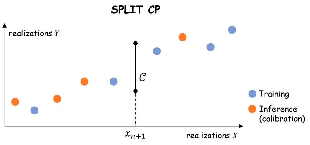
2. Split conformal prediction

Split CP is probably the simplest method achieving finite-sample coverage properties.

Procedure.

Randomly split the dataset ${\mathcal D=\{(x^i,y^i)\}_{1\le i\le n}}$ into training dataset ${\mathcal D^t = \{(x^t_i,y^t_i)\}_{i=1,\dots,n^t}}$ and calibration dataset ${\mathcal D^c=\{(x^c_i,y^c_i)\}_{i=1,\dots,n^c}}$
Train a predictor ${f_{\mathcal D^t}}$ on the training set ${\mathcal D^t}$
Compute the empirical quantile of the residuals on the calibration samples:
$\displaystyle \widehat{q}:=q_{\lceil (1-\alpha)(n^c+1) \rceil}\{|y_i^c-f_{\mathcal D^t}(x_i^c)|\}_{i} \ \ \ \ \ (4)$
Receive the new input ${x_{n+1}}$ .
Return the prediction interval:
$\displaystyle \mathcal C^{\mathrm{split}}(x_{n+1}) = \left[ f_{\mathcal D^t}(x_{n+1}) - \widehat{q}; \, f_{\mathcal D^t}(x_{n+1}) + \widehat{q} \right] \ \ \ \ \ (5)$

The coverage property of split CP directly stems from Theorem 1.

Corollary 2 If the residuals on the calibration samples and the new sample ${(x_{n+1},y_{n+1})}$ are exchangeable, then

$\displaystyle 1-\alpha \le \Pr\left( y_{n+1} \in \mathcal C^{\mathrm{split}}(x_{n+1}) \right) \le 1-\alpha + \frac{1}{n^c+1} \ \ \ \ \ (6)$

where the second inequality holds if the residuals are almost surely distinct.

Pro’s: Split CP has low computational complexity as it only requires to train the predictor ${f}$ once. Moreover, the interval does not need to be recomputed for each different ${x_{n+1}}$ .

Con’s: Split CP may produce a large prediction interval, especially if the dataset is small. In fact, if the training samples are few then the resulting predictor is poor, and its residuals on the calibration samples are large.

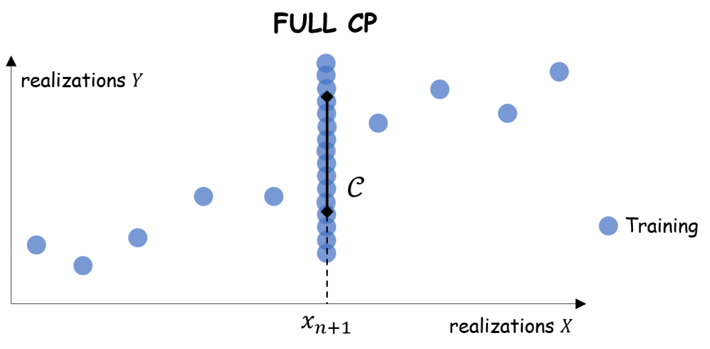
3. Full conformal prediction

We first define ${\widehat{q}^y}$ , for any ${y\in \mathbb R}$ , as the empirical ${(1-\alpha)}$ -th quantile of the residuals with the respect to a regressor trained on the augmented dataset ${\mathcal D \cup (x_{n+1},y)}$ :

$\displaystyle \widehat{q}^y:=q_{\lceil (1-\alpha)(n+1) \rceil}\left\{|y_i-f_{\mathcal D \cup (x_{n+1},y)}(x_i)|\right\}_{i=1,\dots,n}$

Procedure. (Ideal but impractical)

Receive the new input ${x_{n+1}}$ .
Compute the prediction set: $\displaystyle \mathcal C^{\mathrm{full}}(x_{n+1}) = \left\{ y: \, |y - f_{\mathcal D \cup (x_{n+1},y)}(x_{n+1})| \le \widehat{q}^y \right\} \ \ \ \ \ (7)$

A coverage guarantee similar to the one for split CP, still stemming directly from Theorem 1, is achievable for full CP.

Corollary 3 If the residuals on training samples and the new sample ${(x_{n+1},y_{n+1})}$ are exchangeable, then

$\displaystyle 1-\alpha \le \Pr\left( y_{n+1} \in \mathcal C^{\mathrm{full}}(x_{n+1}) \right) \le 1-\alpha + \frac{1}{n+1} \ \ \ \ \ (8)$

where the second inequality holds if residuals are almost surely distinct.

Remark. For the residual exchangeability hypothesis to hold, it is not enough to assume that the samples ${(x_i,y_i)}$ are exchangeable: we also require that regressor ${f}$ be invariant to the order of the training samples. In other words, the regressor should stay unchanged if trained on reshuffled data samples.

Pro’s: Full CP is data efficient, since it trains the regressor on all available historical samples.

Con’s: Full CP is impractical, since it ideally requires infinite computational complexity: the regressor used to decide whether ${y\in \mathcal C^{\mathrm{full}}(x_{n+1})}$ has to be retrained for each different ${y}$ and ${x_{n+1}}$ .

To alleviate the computational complexity issue, one can simply evaluate whether a point ${y}$ belongs to the prediction interval on a discrete grid. However, such procedure, described next, loses the original full CP coverage guarantees.

Procedure. (Practical but approximated)

Define a grid ${y[0],\dots,y[k]}$
Receive the new input ${x_{n+1}}$
Initialize and .
For :
1. Train the regressor ${f_{\mathcal D \cup (x_{n+1},y)}}$
2. Compute the empirical quantile of residuals ${\widehat{q}^y}$
3. If ${|y - f_{\mathcal D \cup (x_{n+1},y)}(x_{n+1})| \le \widehat{q}^y}$ then add ${y}$ to ${\mathcal C^{\mathrm{full}}(x_{n+1})}$ . Otherwise, add ${y}$ to ${\overline{\mathcal C}^{\mathrm{full}}(x_{n+1})}$ .

Finally, to obtain a compact prediction set, one can use the nearest neighbor rule: given ${y}$ , we decide that it belongs to the (approximated) prediction set if the closest element in the grid ${y[0],\dots,y[k]}$ belongs to ${\mathcal C^{\mathrm{full}}(x_{n+1})}$ (and not to ${\overline{\mathcal C}^{\mathrm{full}}(x_{n+1})}$ ).

4. Jackknife+

The intuition behind Jackknife+ [2] is the following. Consider the regressor ${f_{-i}:=f_{\mathcal D \setminus (x_i, y_i)}}$ , trained on the full historical dataset except for the ${i}$ -th sample. If the samples ${(x_i,y_i)}$ , for all ${i}$ , and ${(x_{n+1},y_{n+1})}$ are exchangeable, then the residuals:

${\left|y_i-f_{-i}(x_i)\right|}$ (that we can compute)
${\left|y_{n+1}-f_{-i}(x_{n+1})\right|}$ (that we do not know)

are also exchangeable. Hence, we can exploit the former to learn the distribution of residuals of the new point with respect to the regressor ${f_{-i}}$ , and eventually to learn the typical values of ${y_{n+1}}$ .

Procedure.

For :
- i) train the regressor ${ f_{-i}:=f_{\mathcal D \setminus (x_i, y_i)}}$
- ii) compute the residual ${R_i:=\left|y_i-f_{-i}(x_i)\right|}$
Receive the new input ${x_{n+1}}$
Compute the lower quantile:
$\displaystyle \widehat{q}^- := q_{\lfloor \alpha(n+1) \rfloor}\big\{f_{-i}(x_{n+1}) - R_i \big\}_{i\le n}$
Compute the upper quantile:
$\displaystyle \widehat{q}^+ := q_{\lceil (1-\alpha)(n+1) \rceil}\big\{f_{-i}(x_{n+1}) + R_i \big\}_{i\le n}$
Return the prediction interval:
$\displaystyle \mathcal C^{j+}(x_{n+1})= \left[\widehat{q}^- ; \, \widehat{q}^+ \right] \ \ \ \ \ (9)$

Theorem 4 If the regressor ${f}$ is invariant to the order of training samples and the data points ${\mathcal D\cup (x_{n+1},y_{n+1})}$ are exchangeable, then

$\displaystyle \Pr\left(y_{n+1}\in \mathcal C^{j+}(x_{n+1})\right) \ge 1-2\alpha. \ \ \ \ \ (10)$

Pro’s: Jackknife+ is data efficient as the regressor is trained on the whole dataset (except for a single point). Thanks to this, the produced prediction interval is generally shorter than for split CP, especially if the dataset ${\mathcal D}$ is small.

Con’s: Jackknife+ has a non-negligible computational complexity, especially if the dataset is large. In fact, it retrains the regressor ${n}$ times, where ${n}$ is the size of the historical dataset.

5. Cross-Validation+

To alleviate the complexity issue of Jackknife+, Cross-Validation+ (CV+) [2] first split the historical dataset ${\mathcal D}$ into ${K\le n}$ subsets of equal size, ${\mathcal D_1,\dots,\mathcal D_K}$ . Then, ${K}$ regressors of the kind ${f_{\mathcal D\setminus \mathcal D_k}}$ for ${k=1,\dots,K}$ are trained. Finally, the following prediction interval is produced:

$\displaystyle \mathcal C^{\mathrm{CV+}} = \big[ q_{\lfloor \alpha(n+1) \rfloor}\big\{f_{\mathcal D\setminus \mathcal D_{k(i)}}(x_{n+1}) - R_i^{\mathrm{CV+}} \big\}_{i\le n};$

$\displaystyle \qquad \qquad \qquad q_{\lceil (1-\alpha)(n+1) \rceil}\big\{f_{\mathcal D\setminus \mathcal D_{k(i)}}(x_{n+1}) + R_i^{\mathrm{CV+}} \big\}_{i\le n} \big] \ \ \ \ \ (11)$

where ${k(i)}$ determines the subset containing the ${i}$ -th sample and ${R_i^{\mathrm{CV+}}}$ is the residual on sample ${i}$ with respect to the regressor trained on all subsets except for the ${k(i)}$ -th one:

$\displaystyle R_i^{\mathrm{CV+}} = \left| y_i - f_{\mathcal D\setminus \mathcal D_{k(i)}}(x_i) \right|, \quad \forall\, i=1,\dots,n.$

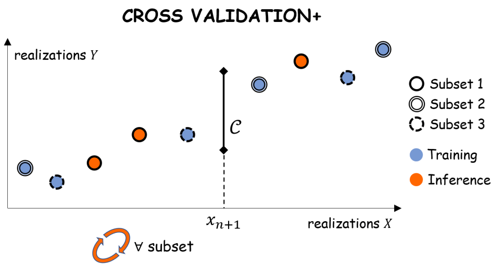
Observe that the Cross-Validation+ procedure boils down to Jackknife+ when ${K=n}$ . As intuition suggests, to choose the number of subsets ${K}$ one must strike a trade-off between complexity and performance: as ${K}$ decreases and the computational burden lessens, the coverage guarantees of Cross-Validation+ worsen. The result below is from [2].

Theorem 5 The Cross-Validation+ prediction interval satisfies:

$\displaystyle \Pr \left( y_{n+1}\in \mathcal C^{\mathrm{CV+}} \right) \ge 1 - 2\alpha - \min\left\{ \frac{2(1-1/K)}{n/K+1}, \, \frac{1-K/n}{K+1} \right\}$

When ${K}$ is small, the first term inside the min operator predominates, while the latter term provides a tighter bound for values of ${K}$ close to ${n}$ . When ${K=n}$ we find the same bound ${1-2\alpha}$ as in Jackknife+, since in this case the two algorithms coincide.

Pro’s: Cross-Validation+ is characterized by a lighter computational complexity than Jackknife+, especially if the number ${K}$ of subsets is small.

Con’s: Cross-Validation+ has worse coverage guarantees than Jackknife+, especially if the number ${K}$ of subsets is small.

6. Other important CP methods

Amongst the other main methods for conformal prediction present in the literature, we mention:

Cross-Validation-minmax and Jackknife+-minmax [2]
Conformalized quantile regression (CQR) [4], already covered in a previous [post]
Jackknife+-after-bootstrap [5]
Ensemble batch prediction intervals (EnbPI) [6]

References

[1] Angelopoulos, Anastasios N., and Stephen Bates. Conformal prediction: A gentle introduction. Foundations and Trends in Machine Learning 16.4 (2023): 494-591.

[2] Barber, R. F., Candes, E. J., Ramdas, A., and Tibshirani, R. J. Predictive inference with the jackknife+. The Annals of Statistics, 49(1):486–507, 2021.

[3] Vovk, Vladimir, Alexander Gammerman, and Glenn Shafer. Algorithmic Learning in a Random World. Springer Nature, 2022.

[4] Romano, Yaniv, Evan Patterson, and Emmanuel Candes. Conformalized quantile regression. Advances in neural information processing systems 32 (2019)

[5] Byol Kim, Chen Xu, and Rina Foygel Barber. Predictive Inference Is Free with the Jackknife+-after-Bootstrap. 34th Conference on Neural Information Processing Systems (NeurIPS 2020)

[6] Xu, Chen et Xie, Yao. Conformal prediction interval for dynamic time-series. In : International Conference on Machine Learning. PMLR, 2021. p. 11559-11569.

[7] Manokhin, V. Awesome conformal prediction [Github repo].

[8] Taquet, V., Blot, V., Morzadec, T., Lacombe, L., Brunel, N. (2022). MAPIE: an open-source library for distribution-free uncertainty quantification. arXiv preprint arXiv:2207.12274. [Python library]

Fifty (four, actually) shades of conformal prediction

Comments

Leave a comment Cancel reply

Fifty (four, actually) shades of conformal prediction

Share this:

Comments

Leave a comment Cancel reply