Conformalized quantile regression

Pimp quantile regression with strong coverage guarantees

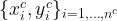
Suppose that we are given a historical dataset containing ${n}$ samples of the form ${\{(x^i,y^i)\}_{1\le i\le n}}$ , where ${x_i\in\mathbb R^d}$ and ${y_i\in \mathbb R}$ are the ${i}$ -th realizations of (predictor) variable ${X}$ and of (predicted) variable ${Y}$ , respectively.

As a running example, let us consider the following dataset:

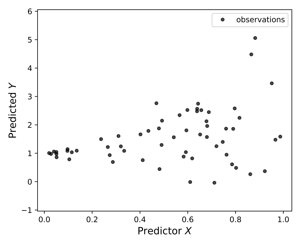
Our goal #1 is to estimate the trend of variable ${Y}$ against ${X}$ while evaluating the uncertainty of our prediction. In other words, point-wise predictions like classic regression do not satisfy us and we aim at to computing intervals where the realizations land with high (say, ${1-\alpha}$ ) coverage probability. More formally, we want to build a set-valued coverage function ${\mathcal C}$ such that, for any new pair of realizations ${(x',y')}$ , it holds that:

$\displaystyle \Pr(y'\in \mathcal C(x')) \approx 1-\alpha, \quad \forall\, n. \ \ \ \ \ (1)$

Our goal #2 is that the length of the prediction interval ${\mathcal C(x)}$ should reflect the local dispersion of ${Y}$ given that ${X=x}$ , for any possible value of ${x}$ . This is especially desirable when the observation noise is heteroscedastic, i.e., its variance depends on the point it is applied to. This happens to be our case, since realizations ${y}$ ‘s are more dispersed as the corresponding ${x}$ ‘s increase.

In this post we show how to achieve goals #1 and #2 via conformal quantile regression (CQR), first proposed by Y. Romano, E. Patterson and E. Candes in [1], which applies conformal prediction (CP) to quantile regression (QR) via a powerful and surprisingly simple-to-implement procedure.

First, let us investigate how QR and “vanilla” CP alone would address our problem, and how each fails to jointly achieve our goals.

1. Via quantile regression (QR)

As explained in a previous post [link], the ${\tau}$ -th quantile regressor ${\widehat{\mathcal Q}^\tau(X)}$ estimates the conditional ${\tau}$ -th quantile ${\mathcal Q^{\tau}[Y|X]}$ of the predicted variable ${Y}$ given the predictor variable ${X}$ .

Then, a natural attempt to build a prediction interval with coverage, ${1-\alpha}$ is the following.

Train a low-quantile regressor ${\widehat{\mathcal Q}^{\frac{\alpha}{2}}}$ on all ${n}$ historical samples
Train a high-quantile regressor ${\widehat{\mathcal Q}^{1-\frac{\alpha}{2}}}$ on all ${n}$ historical samples
Approximate the coverage function as
$\displaystyle \mathcal C^{\mathrm{QR}}(x) = \left[\widehat{\mathcal Q}^{\frac{\alpha}{2}}(x); \, \widehat{\mathcal Q}^{1-\frac{\alpha}{2}}(x)\right], \quad \forall\, x \ \ \ \ \ (2)$

If we apply this procedure to our initial dataset with ${\alpha=0.1}$ (hence, the coverage probability is ${0.9}$ ) using linear QR with polynomial features of order 2, we obtain the following result.

Pro’s: Goal #2 is achieved: ${\mathcal C^{\mathrm{QR}}(x)}$ provides an interval whose length depends on value ${x}$ , which is desirable in the presence of heteroscedastic noise as in our case.

Con’s: Goal #1 is not not achieved. In fact, it holds only asymptotically, as the number of training samples ${n}$ grows to infinity, under some technical assumptions [1].

2. Via vanilla conformal prediction (CP)

We discussed about CP in a previous post [link].

The “vanilla” CP procedure applied to our problem goes as follows:

Randomly split the ${n}$ historical data points into a training set ${\{x_i^t,y_i^t\}_{i=1,\dots,n^t}}$ and a calibration set ${\{x_i^c,y_i^c\}_{i=1,\dots,n^c}}$
Train a least-square regressor ${\widehat{\mathcal L}}$ on the training set
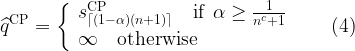
Evaluate the performance of ${\widehat{\mathcal L}}$ on the calibration set by computing the scores:
$\displaystyle s_i^{\mathrm{CP}} = \left|\widehat{\mathcal{L}}(x_i^c) - y_i^c\right|, \quad \forall\, i=1,\dots,n^c \ \ \ \ \ (3)$
Compute the empirical ${(1-\alpha)}$ -th quantile of the scores:
$\displaystyle \widehat{q}^{\mathrm{CP}}= \left\{ \begin{array}{ll} s^{\mathrm{CP}}_{\lceil (1-\alpha)(n+1) \rceil} \quad \mathrm{if} \ \alpha\ge \frac{1}{n^c+1} \\ \infty \quad \mathrm{otherwise} \end{array} \right. \ \ \ \ \ (4)$
Output the coverage function:
$\displaystyle \mathcal{C}^{\mathrm{CP}}(x) = \left[\widehat{\mathcal L}(x)-\widehat{q}^{\mathrm{CP}}; \, \widehat{\mathcal L}(x)+\widehat{q}^{\mathrm{CP}} \right], \quad \forall\, x\in\mathcal{X}. \ \ \ \ \ (5)$

If applied to our initial dataset with a linear least-square regressor using polynomial features of order 2, vanilla CP produces the following result:

Pro’s: Goal #1 is achieved: in fact, under some technical assumptions (see Theorem 2, of our previous post [link]), it holds that, for any new pair of realizations ${(x',y')}$ ,

$\displaystyle 1-\alpha \le \Pr\left(y'\in \mathcal{C}^{\mathrm{CP}}(x') \right) \le 1 - \alpha + \frac{1}{n^c+1}. \ \ \ \ \ (6)$

Con’s: Goal #2 is not achieved: the length of the prediction interval is constant across all values of ${x}$ , which is somehow disappointing especially in the case of heteroscedastic noise, as in our case.

3. Conformalized quantile regression (CQR)

The question arises naturally: Can we take the best of the worlds, QR and CP, and jointly achieve goals #1 and #2?

The answer is yes, via Conformalized Quantile Regression (CQR) [1]. CQR is a direct application of the split CP paradigm to QR, that tweaks the empirical coverage interval ${\mathcal{C}^{\mathrm{QR}}}$ defined in (2) to ensure that its coverage probability is (approximately) ${1-\alpha}$ in the finite samples regime.

CQR Procedure.

Randomly split the ${n}$ historical data points into a training set ${\{x_i^t,y_i^t\}_{i=1,\dots,n^t}}$ and a calibration set ${\{x_i^c,y_i^c\}_{i=1,\dots,n^c}}$
Train a lower quantile regressor ${\widehat{\mathcal Q}^{\frac{\alpha}{2}}}$ on the ${n^t}$ training samples
Train an upper quantile regressor ${\widehat{\mathcal Q}^{1-\frac{\alpha}{2}}}$ on the ${n^t}$ training samples
Computing on the calibration points ${i=1,\dots,n^c}$ the scores:
$\displaystyle s^{\mathrm{CQR}}_i = \max\left\{ y_i^c - \widehat{\mathcal Q}^{1-\frac{\alpha}{2}}(x_i^c), \, \widehat{\mathcal Q}^{\frac{\alpha}{2}}(x_i^c) - y_i^c \right\} \ \ \ \ \ (7)$
Compute the empirical ${(1-\alpha)}$ -th quantile of the scores:
$\displaystyle \widehat{q}^{\mathrm{CQR}} = \left\{ \begin{array}{ll} s^{\mathrm{CQR}}_{\lceil (1-\alpha)(n+1) \rceil} \quad \mathrm{if} \ \alpha\ge \frac{1}{n^c+1} \\ \infty \quad \mathrm{otherwise} \end{array} \right. \ \ \ \ \ (8)$
Output the coverage interval:
$\displaystyle \mathcal{C}^{\mathrm{CQR}}(x) = \left[\widehat{\mathcal Q}^{\frac{\alpha}{2}}(x) - \widehat{q}^{\mathrm{CQR}}; \, \widehat{\mathcal Q}^{1-\frac{\alpha}{2}}(x) + \widehat{q}^{\mathrm{CQR}}\right], \quad \forall\, x. \ \ \ \ \ (9)$

To gather more intuitions, it is instructive to consider the following 3 cases:

Case a): the interval ${\mathcal C^{\mathrm{QR}}}$ built via QR regression only is already conformal. In this case, a portion ${1-\alpha}$ of the calibration samples ${y^c}$ land within ${\mathcal C^{\mathrm{QR}}(x^c)}$ (hence, their score ${s^{\mathrm{CQR}}_i}$ is negative) while the remaining ${\alpha}$ fall outside ${\mathcal C^{\mathrm{QR}}}$ (hence, their score is positive). Thus, the empirical ${(1-\alpha)}$ -th quantile of the scores will be zero and ${\mathcal{C}^{\mathrm{CQR}}=\mathcal{C}^{\mathrm{QR}}}$ .
Case b): ${\mathcal{C}^{\mathrm{QR}}}$ under-covers the calibration samples, i.e., a portion of calibration samples smaller than ${1-\alpha}$ fall inside ${\mathcal{C}^{\mathrm{QR}}}$ . Then, a portion of scores smaller than ${1-\alpha}$ is negative, hence ${\widehat{q}^{\mathrm{CQR}}}$ is positive, hence the resulting interval ${\mathcal{C}^{\mathrm{CQR}}}$ is larger than the non-conformal ${\mathcal{C}^{\mathrm{QR}}}$ .
Case c) ${\mathcal{C}^{\mathrm{QR}}}$ over-covers the calibration samples, i.e., a portion of calibration samples higher than ${1-\alpha}$ fall inside ${\mathcal{C}^{\mathrm{QR}}}$ . Then, following a similar reasoning, the non-conformal ${\mathcal{C}^{\mathrm{QR}}}$ is shrunk to finally obtain ${\mathcal{C}^{\mathrm{CQR}}}$ .

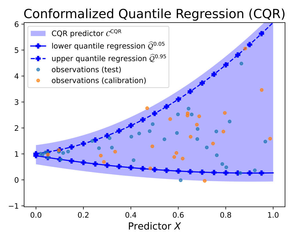
If applied to our initial dataset, CQR provides the following result.

Note that, in this case, the QR interval under-covers calibration samples. In fact, the calibration score distribution is as follows:

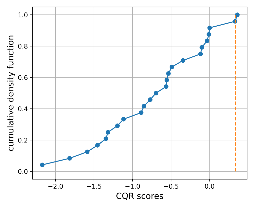
Goal #2 is achieved by CQR, since CQR merely displaces the levels set by the QR regression by a constant offset. We conclude by proving formally that the CQR procedure achieves goal #1 as well, on the coverage probability.

Theorem 1 Let ${(x',y')}$ be a new sample with score ${s'}$ . Suppose that the scores ${s_1,\dots,s_{n^c},s'}$ are exchangeable random variables. Then, the prediction interval ${\mathcal C^{\mathrm{CQR}}}$ satisfies:

$\displaystyle 1-\alpha \le \Pr(y'\in \mathcal{C}^{\mathrm{CQR}}(x')) < 1-\alpha + \frac{1}{n^c+1} \ \ \ \ \ (10)$

where the second inequality holds if the scores are almost surely distinct.

Proof: The event ${y'\in \mathcal{C}^{\mathrm{CQR}}(x')}$ holds whenever

$\displaystyle \left\{ \begin{array}{ll} y' \le \widehat{\mathcal Q}^{1-\frac{\alpha}{2}}(x') + \widehat{q}^{\mathrm{CQR}} \\ y' \ge \widehat{\mathcal Q}^{\frac{\alpha}{2}}(x') - \widehat{q}^{\mathrm{CQR}} \end{array} \right. \ \ \ \ \ (11)$

By rearranging the terms of (11), we obtain the equivalent expression:

$\displaystyle \widehat{q}^{\mathrm{CQR}} \ge \max\left\{ y_i^c - \widehat{\mathcal Q}^{1-\frac{\alpha}{2}}(x'), \, \widehat{\mathcal Q}^{\frac{\alpha}{2}}(x') - y' \right\} := s' \ \ \ \ \ (12).$

It stems that ${\Pr(y'\in \mathcal{C}^{\mathrm{CQR}}(x'))=\Pr(s'\le \widehat{q}^{\mathrm{CQR}})}$ . The thesis follows from Lemma 1 and Theorem 2 of our previous post [link]. $\Box$

3.1. Discussion: Marginal vs Conditional coverage

It is important to understand that the coverage probability ${\Pr(y'\in \mathcal C(x'))}$ in (1), that is required to be approximately ${1-\alpha}$ , is marginalized over the training and calibration samples and, most importantly, over all possible new pairs ${(x',y')}$ . Intuitively, this means that if draw a large number ${m}$ of different calibration samples and of corresponding new points ${\{(x'_i,y'_i)\}_{1\le i \le m}}$ , then for a portion ${1-\alpha}$ of them will lie within the respective coverage interval:

$\displaystyle \frac{|\{y_i': \, y'_i\in \mathcal C(x'_i)\}_{1\le i\le m}|}{m} \ \stackrel{m\uparrow \infty}{\longrightarrow} \Pr(y'\in \mathcal C(x')) \approx 1-\alpha \ \ \ \ \ (13)$

On the other hand, the coverage probability does not hold marginally, i.e., in point-wise fashion:

$\displaystyle \Pr(y'\in \mathcal C(x')) \ne \Pr\left(y'\in \mathcal C(x') \, \big| \, X=x'\right). \ \ \ \ \ (14)$

In other words, if we fix ${X=x'}$ and we draw a large number of realizations of ${Y}$ , the portion of them falling inside ${\mathcal C(x')}$ will be generally different from ${1-\alpha}$ .

This is illustrated below, where we compare the output of CQR with the actual ${90\%}$ (point-wise, i.e., conditional) confidence interval of the distribution that the observations were drawn from.

References

[1] Romano, Y., Patterson, E., Candes, E. (2019). Conformalized quantile regression. Advances in neural information processing systems, 32.

[2] Manokhin, V. Awesome conformal prediction Github repo

Conformalized quantile regression

Pimp quantile regression with strong coverage guarantees

Comments

One response to “Conformalized quantile regression”

Leave a comment Cancel reply

Conformalized quantile regression

Pimp quantile regression with strong coverage guarantees

Share this:

Comments

One response to “Conformalized quantile regression”

Leave a comment Cancel reply