Quantile regression

An expressive and robust alternative to least square

For regression problems, least square regression (LSR) arguably gets the lion share of data scientists’ attention. The reasons are several: LSR is taught in virtually every introductory statistics course, it is intuitive and is readily available in most of software libraries.

LSR estimates the mean of the predicted variable as a function of the value of the observed predictor variable . However, when the dispersion of around its (conditional) mean is considerable, i) LSR generally fails to produce actionable results, since the mean is not informative on the likelihood of extreme values which are the most critical to handle. In this case, a method that can estimate the whole distribution of conditioned on would be preferable.

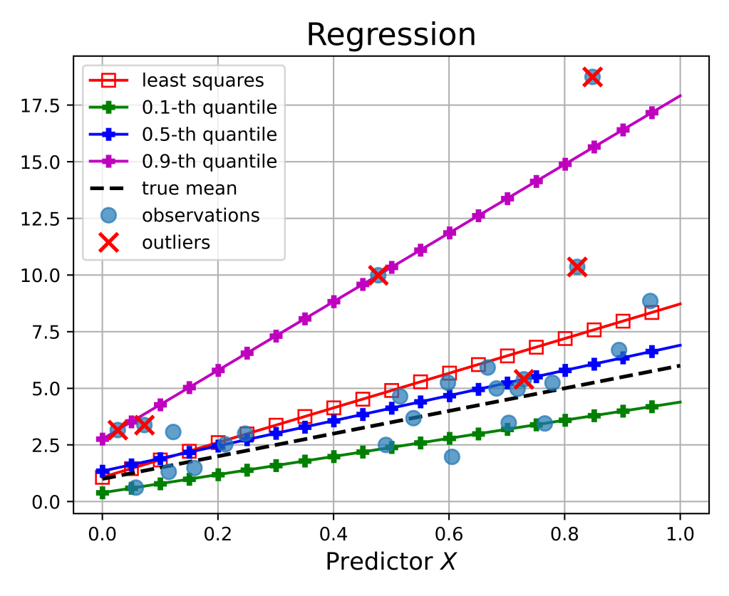
Moreover, ii) LSR is not robust to outliers: the presence of a few “corrupted” points can affect largely the quality of the regression.

Quantile regression (QR) is a method that addresses both concerns i), ii) above: 

i) QR it can estimate any quantile of the distribution of the predicted conditioned on the predictor  

ii) QR is more robust to the presence of outliers than classic LSR.

Next, we first introduce the notion of (conditional) quantile before delving into QR, via an instructive parallel with LSR.

1. Quantile of a random variable

Let consider a random variable , taking on values in . Informally speaking, the -th quantile of is that value that exceeds with probability . For instance, if a person’s height is the -th quantile, it should be then understood that the person is taller than of the population.

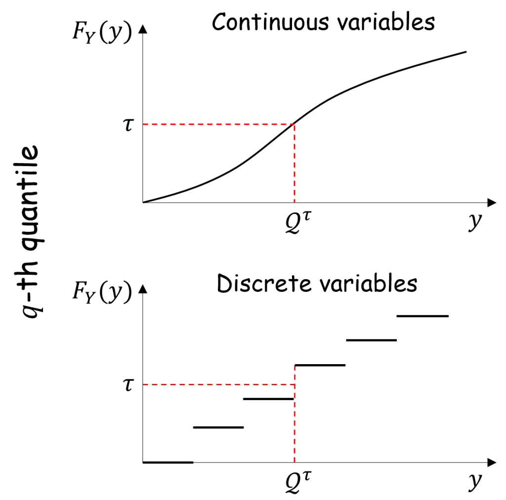
This concept can be directly formalized if the cumulative density function (CDF) is invertible. This holds if is a continuous random variable that can take on any value within an interval. In this case, the -th quantile is such that , i.e.,

However, for discrete variables, the CDF is discontinuous and step-wise constant, hence is not invertible and (1) is not applicable. To understand this, imagine that is a binary variable that takes on values 0 and 1 with probability for each. Then,

Suppose now that we want to compute the -th quantile of . Clearly, cannot be inverted at . It is then clear that a more general definition of quantile is needed.

To cater for non-invertible CDFs, expression (1) is then generalized as the minimum value at which the cumulative density function exceeds .

Definition 1 The -th quantile of random variable is defined as:

Thus, in the example above, the -th quantile of the binary variable is effectively 1.
Note also that, when is invertible, then definition (3) boils down to (1).

Estimation. In most practical cases, we do not have access to the CDF . Instead, we can rely on a historical dataset containing independent realizations of the random variable . In this case, the -th quantile can be estimated as the -th worst realization. If we suppose that the realizations are sorted in increasing order (), the sample quantile equals:

Conditional quantile. Extending the definition of quantile to conditioned random variables is straightforward. Suppose that is correlated with another variable , called predictor, that is observed and takes on values within where . We call the CDF of the variable conditioned on the observed value of . Then, the conditional -th quantile  is defined similarly to (3).

Definition 2 The -th conditional quantile of random variable given variable is defined as:

2. Regression: Quantile vs. Least square

The goal of regression is to estimate a predefined target statistics of the predicted variable upon observing a realization of the predictor variable .

• If such statistic is the conditional mean, i.e., , then we obtain the classic least square regression (LSR);
• If such statistic is the -th conditional quantile, i.e., , then we obtain the quantile regression (QR).

Assume now that we have observed independent joint realizations of variables and , denoted as .

A naive approach for quantile regression would prescribe, for each , to aggregate observations pairs where the predictor variables takes on the same value and to apply the formula for the sample quantile (4) to the corresponding values ‘s. However, this method fails miserably if is a continuous variable, whose realizations are almost surely distinct; in this case, one would end up computing sample quantiles over… one sample!

A better (but still unsatisfactory) approach would be to cluster the observations into bins where the values are “close”, and compute (4) for each bin. Yet, this method is not scalable as the number of dimensions of variable grows large.

To introduce QR, let us make a step back to analyze general (hence, not necessarily quantile) regression problems.

Let be a “guess” for the desired statistic . In other words, if it has been observed that , then guesses the statistic . Then, the regression procedure is as follows.

1. Design a loss function  such that the guess function that minimizes the expected loss is precisely the target statistic :
   
   Recall that is to be meant as a function that, for each possible value , produces the statistic of predicted variable given that the predictor takes on value .
2. Define a parametrized class of functions  where is the vector of parameters.
   • If , where is the -th component of , then the regression is linear;
   • In case of deep learning, is the collection of weights and biases of a neural network.
3. Minimize the empirical loss:
   
   where is a potential regularizer, that penalizes extreme values of (e.g., ).
   Finally, is our regressor.

Next we discuss how to go about steps 1 and 3 in the case of LSR and QR.

2.1. Loss function design

To design the appropriate loss function for QR, it is instructive to draw a parallel with its more popular LSR counterpart.

Least squares regression (LSR) draws its name precisely from its loss function, being the square of the residual :

The loss function , to be minimized, entices the guess to stay as close as possible to the true value . It is then intuitive that, out of all possible functions mapping to , the expected LSR loss is minimized by the conditional mean , as prescribed by expression (6).

Theorem 3 The conditional mean , meant as a function that maps each to , minimizes the expected loss:

where the expectation is with respect to the joint distribution of and .

Proof: We first prove that, for any fixed and for all ,

Hereafter, for simplicity of notation we will omit the dependency on . Then, we obtain:

The second term is nonnegative since , while the third term is null since . It stems that (10) holds. The thesis follows from taking the expectation of both terms of (10) with respect to the predictor .

Quantile regression (QR). Similarly to the LSR case, the loss function for the -th QR shall be designed as that function whose expectation is minimized by the -th quantile . It turns out that, as we will prove next, the desired loss function writes:

Note that, in contrast to LSR, residuals are weighted differently depending on their sign. Moreover, the loss function increases only linearly with the magnitude of the residuals. Interestingly, when our target statistic is the conditional median (i.e., ), then the loss simply equals the absolute residual.

Theorem 4 The conditional quantile , meant as a function that maps each to , minimizes the expected loss:

Proof: We prove the thesis under the assumption that the CDF is invertible. Similarly to Theorem 3, we first prove that, for any fixed and for all ,

By omitting the dependency on for notation simplicity and after unfolding the expectation, (15) becomes:

To prove (16) we will take the derivative of the function to be minimized with respect to and set it to 0. Leibniz integration rule, that we report here below, comes in handy:

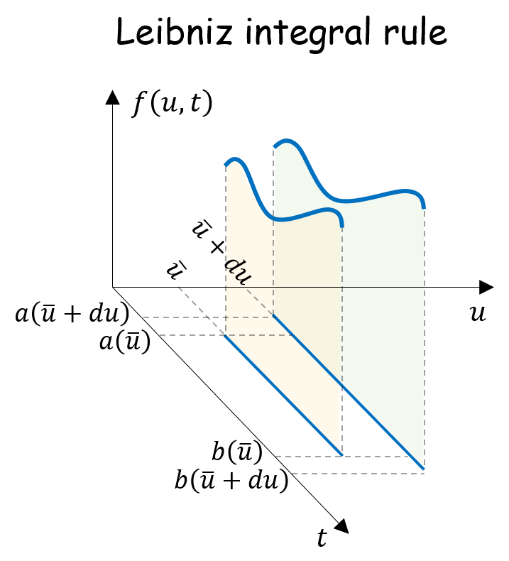
By applying Leibniz rule to the terms in (16) we obtain:

Thus, the optimal , which proves (16) and (15). The thesis follows form taking the expectation of both terms of (15) with respect to .

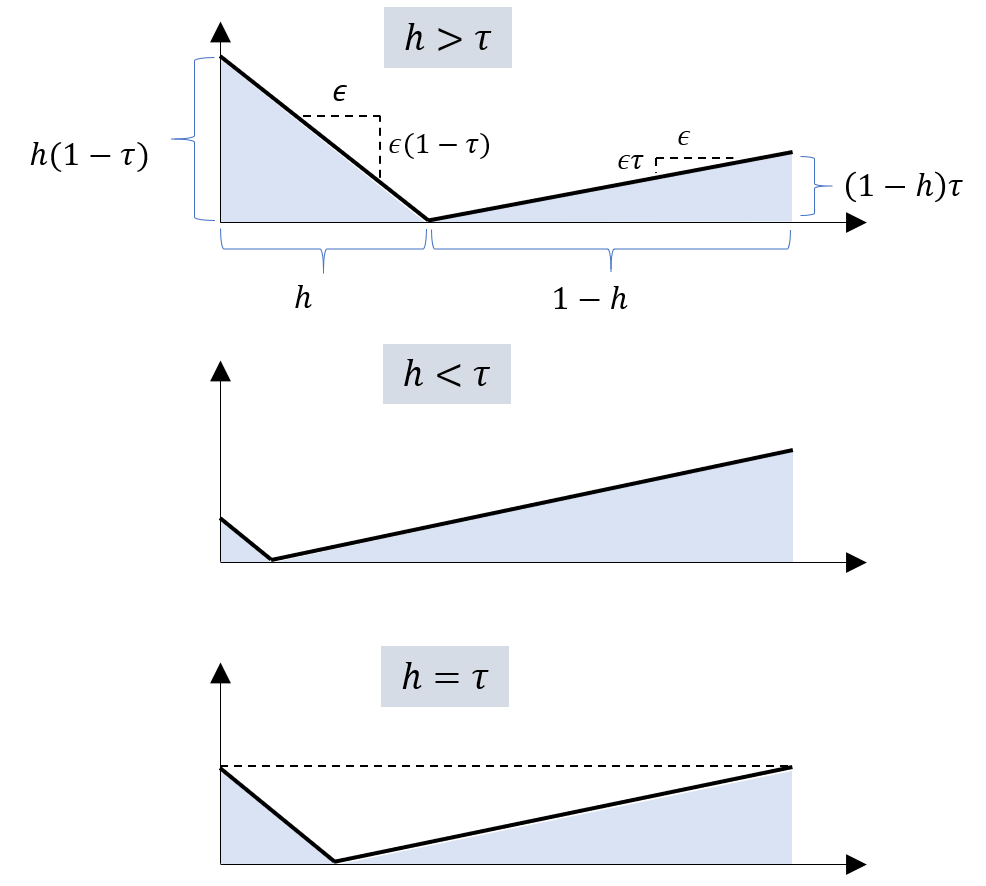
To gain some visual intuitions of the result of Theorem (4), it is useful to consider the simple case where is not considered and is a uniform variable between 0 and 1. In this case, equation (14) boils down to:

By taking the derivative with respect to and setting it to 0 we obtain, as expected, that the optimal is indeed :

2.2. Empirical loss minimization

For simplicity, we here confine ourselves to linear regression, where the guessing function takes the form:

Also, we discard the regularizer, and we aim at solving the empirical average of losses:

Finally, our -th quantile regressor will be .

Least square regression (LSR). If the loss in (24), then we can rewrite the problem as:

where is the column vector of observations of the predicted and is the matrix of observations of the predictor , whose -th column (multiplying ) contains the observations of the -th predictor variable. By computing the derivative of (26) with respect to and setting it to 0 we obtain the classic linear LSR formula:

When non-linear regression is used, in general there exists no closed-form formula for , which has to be computed or approximated via numerical methods.

Quantile regression (QR). Even for linear QR, no closed-form formula for the optimal exists. One can rather compute it via linear programming, as we show next.

We first rewrite the residual , where is its positive part, i.e., , and is its negative part, i.e., . Then, we can re-express the empirical loss minimization problem (24), with , as the following linear program:

3. Robustness to outliers

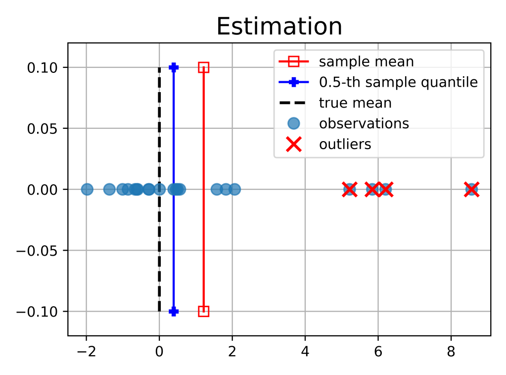
Real data are often messy and may contain extreme “corrupted” values, commonly called outliers. It turns out that both quantile estimation and regression are robust to outliers. We provide some intuitions below.

Estimation. Let us start with the simpler case where the predictor variable is absent, and the -the quantile is estimated as the -th worst realization of variable , as in (4). In this case, even if we corrupt the dataset samples with arbitrary large outliers, as long as their number does not exceed , then the sample quantile will still lie within the original, uncorrupted set of values. More formally, we say that the breakdown point of is , which tends to as tends to infinity.

In contrast, the sample mean is not robust to outliers. In fact, by corrupting a single data point, one can let the sample mean take on an arbitrary value. Equivalently, we say that the breakdown point of the sample mean is 0.

Importantly, if the distribution of is symmetrical around its mean, then the -th quantile, also called median, coincides with the mean. This suggests that, in this case, the sample median is a more robust estimator for the mean than the sample mean itself.

Regression. Once again, it is instructive to draw a parallel between QR and LSR. In the loss function of LSR (8), residuals are squared: if an outlier has a residual being 4 times larger than a non-outlier, then its associated loss is 16 times bigger. On the other hand, the loss in QR (13) is simply proportional to the residual magnitude, hence the outlier would incur a loss being only 4 times higher than the non-outlier.

As a result, in the quest for minimizing its loss, LSR has the natural tendency to “over-react” to the presence of outliers by bringing closer to outliers than QR. In the figure below we demonstrate this on numerical examples, produced via scikit-learn [4], where we compare LSR to its alter-ego: the median regression, i.e., the -th QR.

References

[1] Koenker, R. (2005). Quantile regression (Vol. 38). Cambridge university press.

[2] Hao, L., Naiman, D. Q. (2007). Quantile regression (No. 149). Sage.

[3] Scikit-learn Quantile Regressor examples

[4] Scikit-learn Quantile Regressor function

[5] Stackexchange: Formulating Quantile Regression as a Linear Program