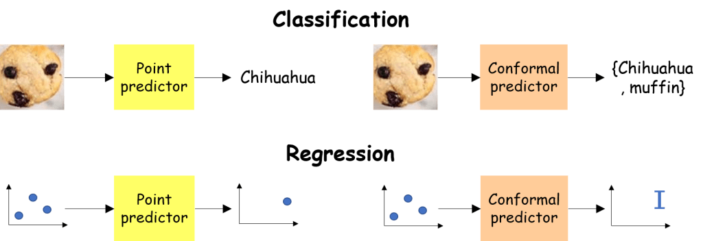
Make any predictor uncertainty-aware via conformal prediction

The importance of being uncertainty-aware. When making a prediction (in a regression or a classification setting) based on observed inputs ${X}$ , it is often important to know which range ${[\underline{Y},\overline{Y}]}$ the true value ${Y}$ will fall in, with high confidence.

For instance, a trader would be interested in knowing within which boundaries the stock price remains, rather than a single “best guess” price, to anticipate the next move. Else, a doctor examining an MRI (Magnetic Resonance Image) scan would want to know whether a certain illness can be confidently ruled out, and if not, take the necessary actions.

This can be generally achieved via Bayesian models, that assign probability distributions to the model parameters that are updated via Bayes formula as new data is observed.

Although the Bayesian viewpoint has been gaining traction in the last few years, the bulk of ML models out there are still uncertainty-unaware, and point-based. Indeed, after observing the next input ${X'}$ , the point-predictor will only output only a single value ${\hat{Y}}$ , being its best guess for ${Y'}$ .

An elegant method called conformity prediction [1]-[5], based on simple intuitions and math, is able to quantify the uncertainty of any point predictor, with surprisingly low additional effort.

Scenario. Let ${f:X\rightarrow Y}$ be a predictor observing input ${X}$ and providing a “best guess” ${Y=f(X)}$ . The predictor has been trained on a subset of the historical data, containing ${n}$ i.i.d. pairs ${\{(X_i,Y_i)\}_{i=1,\dots,n}}$ . A new pair ${(X',Y')}$ is drawn independently from the same distribution. The input ${X'}$ is observed, while the corresponding ${Y'}$ is unknown.

Goal: Coverage. Given a miscoverage level ${\alpha\in(0,1)}$ , we want to produce a set ${\mathcal{C}(X')}$ that is ensured to contain the true (and unknown) ${Y'}$ with (roughly) probability ${1-\alpha}$ . More formally,

$\displaystyle 1-\alpha \le \Pr\left(Y' \in \mathcal{C}(X')\right) \le 1 - \alpha + h(n). \ \ \ \ \ (1)$

where ${h(n)\rightarrow 0}$ as ${n\rightarrow \infty}$ .

A first (dumb) attempt. Imagine that ${\mathcal{C}(X')}$ equals with probability ${1-\alpha}$ the whole set ${\mathcal Y}$ that ${Y'}$ can possibly belong to, and the empty set ${\emptyset}$ otherwise. Then, (1) is clearly satisfied, but we are definitely not!

Small set property. The example above hints at the fact we not only want to fulfill (1), but we intuitively want ${\mathcal{C}(X')}$ to be actionable, hence of “small” size. More specifically, the size of ${\mathcal{C}(X')}$ should depends on the hardness of the problem. In other words, the higher the miscoverage ${\alpha}$ is (i.e., the “easier” the problem), the smaller ${\mathcal{C}(X')}$ should be.

A second (smarter) attempt. Let us consider regression problems, where the input ${X\in \mathbb{R}^d}$ and the output ${Y\in \mathbb R}$ live in their respective Euclidean spaces. A method widely used in practice to approximate ${\mathcal{C}(X')}$ is to

train the predictor ${f}$ on all ${\{(X_i,Y_i)\}_{i=1,\dots,n}}$ pairs
compute the residuals ${r_i=|Y_i-f(X_i)|}$ , ${i=1,\dots,n}$
compute the ${(1-\alpha)}$ quantile of the empirical distribution of ${r_i}$ , that we call ${\widetilde{q}}$
output the prediction interval ${[f(X')-\widetilde{q}; f(X')+\widetilde{q}]}$

Although intuitively sound, such procedure is approximately valid only for a large number of samples, and under certain regularity conditions on the underlying data distribution and the estimator ${f}$ itself [3]. In practice, for small number of samples the prediction interval can flagrantly undercover the true value ${Y'}$ , since the empirical distribution of the residuals counts few extremal values.

The main intuition. In the attempt above, there exists a fundamental difference between the points ${(X_i,Y_i)}$ in the historical dataset and the new point ${(X',Y')}$ : the former ones are used to train the predictor ${f}$ , while the latter is not.

Instead, suppose that we randomly split the first ${n}$ points into two sets of size ${n^t}$ and ${n^c}$ : the training and the calibration set, respectively. On the former we effectively train ${f}$ , while on the latter we simply test its performance. Then, the ${n^c}$ calibration points and the new point ${(X',Y')}$ effectively stand on the same footing, since they equally do not participate in the training of ${f}$ , and are all drawn from the same distribution. Thus, if we now compute the empirical ${(1-\alpha)}$ quantile of the residuals on the calibration set, called ${\widehat{q}}$ , we can reasonably hope that ${Y'}$ falls into ${[f(X')-\widehat q; f(X')+\widehat q]}$ with probability ${1-\alpha}$ , as any other calibration point!

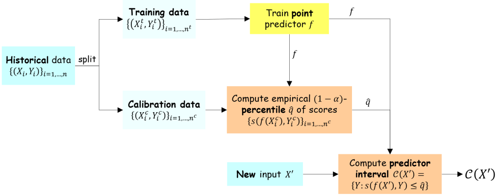
Next, we detail the main steps of conformal prediction in the general setting covering regression and classification problems. Finally, we prove its properties.

Conformal prediction procedure. Consider a prediction (regression or classification) problem. Given a historical dataset of ${n}$ i.i.d. pairs ${\{(X_i,Y_i)\}_{i=1,\dots,n}}$ and a miscoverage target ${\alpha\in(0,1)}$ , follow the steps:

Determine a score function ${s(f(X),Y)}$ ; lower scores correspond to better predictions
Randomly split the dataset into training dataset ${\{(X^t_i,Y^t_i)\}_{i=1,\dots,n^t}}$ and calibration dataset ${\{(X^c_i,Y^c_i)\}_{i=1,\dots,n^c}}$
Train a predictor ${f}$ on the training set
Compute the scores ${\{s(f(X_i^c),Y_i^c)\}_i}$ obtained by the predictor on the calibration set and sort them in increasing order: ${s_1\le \dots\le s_{n^c}}$
Compute the empirical ${(1-\alpha)}$ -quantile of the scores: $\displaystyle \widehat{q}= \left\{ \begin{array}{ll} s_{\lceil (1-\alpha)(n^c+1) \rceil} \quad \mathrm{if} \ \alpha\ge \frac{1}{n^c+1} \\ \infty \quad \mathrm{otherwise} \end{array} \right. \ \ \ \ \ (2)$
Receive the new input ${X'}$ . Compute the prediction interval:
$\displaystyle \mathcal C(X') = \left\{ Y: \, s(f(X'),Y)\le \widehat{q} \right\} \ \ \ \ \ (3)$

If the true value ${Y'}$ is finally observed, then we can add the pair ${(X',Y')}$ to the training set (hence, possibly re-train ${f}$ ) or to the calibration set (hence, possibly recompute ${\widehat{q}}$ ), and reiterate.

Properties. We first observe that the conformal predictor fulfills the small set size property: the higher the miscoverage ${\alpha}$ is (i.e., the “easier” the problem), the smaller ${\mathcal{C}(X')}$ is, by its definition.

We now show formally that ${\mathcal{C}(X')}$ satisfies the coverage property (1). For the sake of simplicity we will assume that score ties never happen (which can be obtained by adding a small noise, if necessary).

We start from an intuitive result.

Lemma 1 Assume that the scores ${s_1,\dots,s_{n^c},s'}$ are almost surely distinct and exchangeable, i.e., their joint distribution is not affected by a permutation of the variables. Then,

$\displaystyle \Pr(s'\le s_k) = \frac{k}{n^c+1}. \ \ \ \ \ (4)$

Proof: We first compute the probability that the score ${s':=s(f(X'),Y')}$ falls in any of the ${(n^c+1)}$ intervals:

$\displaystyle I_0=(-\infty, s_1], \ I_1=(s_1,s_2], \ \dots , \ I_{n^c}=(s_{n^c},\infty)$ . Then, by assumption,

$\displaystyle \Pr(s'\in I_k) = \frac{{n^c \choose k} k! (n^c-k)!}{(n_c+1)!} = \frac{1}{n^c+1} \ \ \ \ \ (5)$

where ${{n^c \choose k}}$ is the number of unordered ways that one can split the ${n^c}$ scores in two parts of size ${k}$ and ${n^c-k}$ (at the left and at the right side of ${s'}$ ), respectively; ${k!}$ and ${(n^c-k)!}$ count the number of permutations in the left and right part, respectively, and ${(n_c+1)!}$ is the total number of combinations. Thus,

$\displaystyle \Pr(s'\le s_k) = \sum_{i=0}^{k-1} \Pr(s'\in I_i) = \frac{k}{n^c+1}. \ \ \ \ \ (6)$ $\Box$

We remark that i.i.d. variables are also exchangeable. Thus, the exchangeability assumption is looser than the i.i.d. one.

It is perhaps suprisingly easy to derive from Lemma 1 that the conformal prediction fulfills the coverage property (1), as we show below.

Theorem 2 If the scores are exchangeable, then the prediction interval ${\mathcal C}$ defined in (3) satisfies:

$\displaystyle 1-\alpha \le \Pr(Y'\in \mathcal{C}(X')) < 1-\alpha + \frac{1}{n^c+1} \ \ \ \ \ (7)$

where the second inequality holds if the scores are almost surely distinct.

Proof: If ${\alpha<\frac{1}{n^c+1}}$ , then ${\widehat{q}=\infty}$ and we trivially obtain ${1-\alpha\le \Pr(Y'\in \mathcal C(X'))\le 1}$ . Otherwise, by the definition of ${\mathcal C (X')}$ , we have

$\displaystyle \Pr \left( Y'\in \mathcal{C}(X') \right) = \Pr\left( s(f(X'),Y')\le \widehat{q} \right) \ \ \ \ \ (8)$

$\displaystyle \qquad = \Pr\left( s(f(X'),Y')\le s_{\lceil (1-\alpha)(n^c+1) \rceil} \right) \ \ \ \ \ (9)$

$\displaystyle \qquad = \frac{\lceil (1-\alpha)(n^c+1) \rceil}{n^c+1} \ \ \ \ \ (10)$

where (10) stems from Lemma 1. By bounding the quantity above as:

$\displaystyle \frac{(1-\alpha)(n^c+1)}{n^c+1} \le \frac{\lceil (1-\alpha)(n^c+1) \rceil}{n^c+1} \le \frac{(1-\alpha)(n^c+1) +1}{n^c+1} \ \ \ \ \ (10)$

we retrieve (7), as desired. $\Box$

In pratice, the assumption of scores being distinct is not restrictive; in the case that they are not distinct, it suffices to add a (small) i.i.d. noise term to the calibration points and to the new point as well to let the result above hold.

Finally, to satisfy the coverage property (1), it suffices to let the size of the calibration set ${n^c}$ grow, e.g., linearly, with ${n}$ . In other words, a certain (small) portion of the historical data is reserved to calibration.

That’s (not) all folks! This post covers the main principles underpinning the early work by Vovk et al. [1,2]. However, this post is far from exhaustive and does not include more recent advances on adaptive prediction sets, group balancedness, outlier detection, etc. that one can find in, e.g., [3].

References

[1] Vovk, V. Gammerman, A., Shafer, G. (2005). Algorithmic Learning in a Random World. Springer.

[2] Shafer, G., Vovk, V. (2008). A Tutorial on Conformal Prediction. Journal of Machine Learning Research, 9(3).

[3] Angelopoulos, A. N., Bates, S. (2021). A gentle introduction to conformal prediction and distribution-free uncertainty quantification. arXiv preprint arXiv:2107.07511.

[4] Lei, J., G’Sell, M., Rinaldo, A., Tibshirani, R. J., Wasserman, L. (2018). Distribution-free predictive inference for regression. Journal of the American Statistical Association, 113(523), 1094-1111.

[5] https://github.com/valeman/awesome-conformal-prediction

Make any predictor uncertainty-aware via conformal prediction

Comments

One response to “Make any predictor uncertainty-aware via conformal prediction”

Leave a comment Cancel reply

Make any predictor uncertainty-aware via conformal prediction

Share this:

Comments

One response to “Make any predictor uncertainty-aware via conformal prediction”

Leave a comment Cancel reply