Is Reinforcement Learning all you need?

When attacking a new problem, the algorithm designer typically follows 3 main steps:

1. First, rule out options that are unlikely to work well
2. Then, test the handful of options that made the first cut
3. Finally, pick the best one and polish it until it shines

When reporting her/his work, the algorithm designer will proudly focus on step 3), briefly mention 2) and likely sweep 1) under the carpet. Yet, skimming alternatives off is a crucial step, that inevitably impacts (positively or negatively) months of hard work on testing and polishing.

With this note, I would like to lift the veil on step 1) and start sharing some subjective, but hopefully relatable, insights on how to navigate through the staggering amount of options available to the algorithm designer to solve a sequential decision-making problem.

Model your problem

The most widespread model for sequential decision making them is Markov Decision Processes (MDP). We will next focus on problems that can be modeled as an MDP and navigate through some options available to actually solve them. Before that, we will provide an (informal) of MDP.

MDPs describe the interaction between an optimizing “agent” and the “environment” across multiple time steps. At step ,

• the agent observes the “state”  of the environment
• the agent takes an “action”  according to some (possibly random) strategy
• the agent receives a (possibly stochastic) instantaneous reward  
• the environment transitions to a new state  with probability , depending on both the current state  and on the agent’s action

and the process is repeated across steps. The agent’s goal is to maximize the Long-Term (LT) sum of rewards:

  (LT)

where the expectation is with respect to the agent’s strategy and the environment state evolution, and  is a math trick avoiding the sum to blow up to infinity and determines the agent’s bias between short-term and long-term payoffs.

The recent popularity of MDPs rides Reinforcement Learning’s (RL) coattails. RL is a class of techniques allowing an agent who has (initially) no clue about the environment behavior, namely the reward function and the state transition rule, to maximize its long-term reward by only observing the sequence of states and rewards.

Given the great generality of MDPs and the tremendous promise that RL holds, it is tempting to think that RL as the “holy grail” of optimization techniques. However, selecting the appropriate algorithm for the problem at hand is a multi-criteria decision problem per se, where factors as convergence speed, robustness, computational (hence, financial) cost, maintenance effort, compliancy with legacy infrastructure, and…performance must be accounted for altogether.

Ad-hoc techniques can arguably strike a better trade-off on the aforementioned factors than “full-blown” RL, depending on a few characterizing traits of the use case at hand that we discuss next.

Navigate through the options

Importantly, we will hereafter assume that our problem can be modeled as an MDP, defined by the tuple state/reward/action/transition as above.

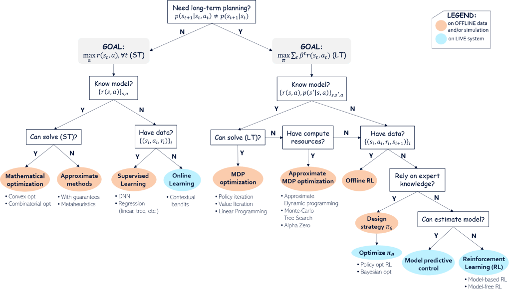
Remember that our goal here is to rule out the bulk of the options available and shortlist a handful of candidate algorithm to solve our problem. The decision tree below translates the proposed mental process we can follow to navigate through the staggering breadth of alternatives available to us, which have been developed by some of the most brilliant minds of the last century.

Short- vs Long-term planning

The first question we shall ask is whether we need long-term planning in the first place. In other words, in order to solve the original long-term problem (LT), we wonder if we can settle to find the short-term (myopic) policy maximizing the instantaneous reward in each single state, namely:

(ST)

which coincides with (LT) when . Trading (LT) with its short-term version (ST) is legitimate when, for instance, the actions do not influence the evolution of states over time, or more formally, when  for any action and states . In this case, the action  taken in current state  only has an impact on the instantaneous reward , so there is no reason to plan ahead.

We realize that (ST) is by far simpler than its long-term counterpart (LT) for the following reasons:

1. The search space of (LT), namely the set of possible strategies , is considerably smaller than for (LT). In (LT), since the action taken in one state impacts the future course of states, actions must be optimized jointly across all states, leading to a total number of strategies being exponential in the number of states (that itself can be huge!). On the other hand, in (ST) one can afford to optimize actions in each state independently, bringing the search space size down from exponential to linear in the number of states.
2. The (ST) formulation does not depend on the state transition law  which, irrespective of its complexity, can be completely neglected for the purpose of maximizing rewards.
3. In (ST) one can immediately assess the “quality” of an action by observing the instantaneous reward, hence promptly making up for bad decisions. In contrast, in (LT) it is not immediately obvious how to evaluate an action, since its impact can only be assessed over the long-term. This naturally leads to longer learning time scales, hence to slower convergence towards a good strategy.

Short-term planning: Mathematical optimization

Here we are with our first, and often immediately obvious, option for solving our problem.

Suppose that, prior to any interaction with the real system, we have the luxury of knowing (or reliably estimating)the “model”, namely the analytical expression of the reward function, mapping state and action pairs to the instantaneous reward .

In this case, one can find the optimal strategy in offline fashion, without the need ofinteracting with the “live” environment, on which trial-and-error exploration can be risky. Rather, we can solve the short-term problem (ST) via a “classic” mathematical optimization. To pinpoint the best technique, the first question to ask is whether , meant as a function of action , is continuous or discrete. In the former case, the next distinction to make is between convex [1] and non-convex [2] optimization; in the latter, we will need to step into the world of combinatorial optimization [3], approximation algorithms [4], and metaheuristics [5].

Short-term planning: Supervised Learning

Suppose now that the “model”  is unknown to us. To still try and avoid any potentially risky “online” (additional) interaction with the live system, the next question we shall ask is whether offline historical data are available, reporting the reward obtained when the system was in state  and action was used at different time steps indexed by .

Then, we can reconstruct the input/output reward relation  via supervised learning. To this aim, we first define a function approximator  depending on parameters  (say, the weights and biases of a neural network) and optimize  by minimizing, e.g., the square loss between the predicted/interpolated value and the actually observed one:

Finally, to compute the (approximately) optimal strategy, we maximize the obtained reward  over actions  in each state  via mathematical optimization as in the paragraph above.

Short-term planning: Online Learning

If we have no clue on the reward function and we have no or insufficient historical data, then we must resort to look for the optimal strategy by interacting online with the environment, that returns the reward  each time the agent chooses action  in state .

The main challenge is converging to the optimal strategy as quickly as possible, hence limiting the (necessary!) trial-and-error learning process which can degrade the possibly fragile live environment that the agent interacts with.

Since we are still in the short-term scenario, we do not care about learning the state evolution law, but only the reward function. In this case, multi-armed bandit algorithms [6] suits our general purpose. The challenge is resolving the exploration-vs-exploitation dilemma: on the one hand, we want to sample actions that, given previous interactions with the environment, are likely to perform well (exploitation). On the other hand, we want to avoid missing untapped opportunities for unexplored actions (exploration). Bandit algorithms solve this dilemma with the aim of minimizing the regret of not having chosen the a-posteriori optimal actions and, eventually, maximizing the convergence speed towards the optimal strategy.

If similar actions are supposed to provide similar rewards in similar states, then one can assume some continuity property of the reward function  and use contextual bandits [7] to crucially increase the convergence speed of the learning process by interpolating  from few past samples.

Long-term planning: Approximate MDP optimization

Classic MDP solution methods suffer from the classic curse of dimensionality and are impractical when the number of states and actions is large. To alleviate this, a number of approximate methods have been developed, ranging from Approximate Dynamic Programming (ADP) [10] to Monte-Carlo Tree Search (MCTS) [11] and its most famous successor Alpha-Go [12], mastering the game of Go.

ADP is about approximating the strategy and/or the long-term reward (more precisely, value function) via parametric functions and optimizing the corresponding parameters. MCTS and Alpha-Go offer instead a principled way to navigate through the huge tree of possibilities that open up to the agent at each step; however, they are tailored to problems possessing a final state (e.g., the end of a game). Moreover, MCTS and Alpha-Go need to interact with an emulator of the system, behave in compliance with the known “model”.

Such methods still require a considerable amount of computational resources and rely on the (sometimes debatable) assumption that the model is known in the first place.

Long-term planning: Offline Reinforcement Learning

Imagine now that the model is unknown, else it is known but neither the exact nor the approximate MDP solution is affordable given our compute resources. Then, our last “offline” option before resorting to online optimization consists in tapping into (if any) available historical data reporting tuples of state , action , reward , and subsequent state  at different past time steps .

Offline Reinforcement Learning [13] is a nascent and exciting research field holding the promise of computing the (approximate) optimal strategy only from historical data. However, practical limitations are still significant, and mainly stem from the impossibility of making counterfactual arguments (i.e., what if a different action had been picked?).

Long-term planning: Relying on domain expert knowledge

If model is unknown, or known but intractable, or not sufficient data is not available, then we must accept to optimize the strategy by interacting with the live environment. Before resorting to “full-blown” RL, we still have the option of interrogating the application domain experts having years of hands-on experience. They may not help to reconstruct an MDP model but can likely provide excellent intuitions on what kind of strategies may work well in practice.

If our priority is learning a decent solution quickly rather than the optimal one with lots of trails and errors, then we can try and craft with the aid of domain experts a class of reasonable policy that depend on a number of parameters. For instance, such parameters can be in the form of thresholds (i.e., the selected action in a state depends on how a certain state component compares with respect to a certain threshold).

To optimize such parameters, we have two main options: policy optimization RL and black-box optimization. The former exploits the assumption that there exists an underlying (unknown) MDP and steers the parameter value along the gradient of the long-term reward [14] or by ensuring that the policy remains in a trusted, safe region [15-16]. The latter option instead makes no assumption on the underlying model [17] and use statistical methods that solve the exploration-vs-exploitation dilemma such as, e.g., Bayesian optimization [8].

Long-term planning: Reinforcement Learning

Last but not least, if we do not settle for hand-crafted policies and we shoot for top performance without any serious concerns on strategy exploration on the live environment, we shall finally turn to “full-blown” online Reinforcement Learning (RL), as popularized by [18], [19].

Within RL, we find two main classes of algorithms, model-based and model-free. In the former, the “model” is learnt by interacting with the environment and used to guess the optimal policy. The latter includes policy optimization as discussed in the previous section, but where the class of parameterized policies is not hand-crafted but rather defined by a general function approximator, e.g., a neural network.

References

[1] Boyd, S. P., & Vandenberghe, L. (2004). Convex optimization. Cambridge University Press.

[2] Kochenderfer, M. J., & Wheeler, T. A. (2019). Algorithms for optimization. MIT Press.

[3] Papadimitriou, C. H., & Steiglitz, K. (1998). Combinatorial optimization: algorithms and complexity. Courier Corporation.

[4] Vazirani, V. V. (2001). Approximation algorithms (Vol. 1). Springer.

[5] Gendreau, M., & Potvin, J. Y. (Eds.). (2010). Handbook of metaheuristics (Vol. 2, p. 9). New York: Springer.

[6] Lattimore, T., & Szepesvári, C. (2020). Bandit algorithms. Cambridge University Press.

[7] Chu, W., Li, L., Reyzin, L., & Schapire, R. (2011, June). Contextual bandits with linear payoff functions. In Proceedings of the Fourteenth International Conference on Artificial Intelligence and Statistics (pp. 208-214). JMLR Workshop and Conference Proceedings.

[8] Shahriari, B., Swersky, K., Wang, Z., Adams, R. P., & De Freitas, N. (2015). Taking the human out of the loop: A review of Bayesian optimization. Proceedings of the IEEE, 104(1), 148-175.

[9] Puterman, M. L. (2014). Markov decision processes: Discrete stochastic dynamic programming. John Wiley & Sons.

[10] Powell, W. B. (2007). Approximate Dynamic Programming: Solving the curses of dimensionality (Vol. 703). John Wiley & Sons.

[11] Kocsis, L., & Szepesvári, C. (2006, September). Bandit based monte-carlo planning. In European conference on machine learning (pp. 282-293). Berlin, Heidelberg: Springer Berlin Heidelberg.

[12] Silver, D., Huang, A., Maddison, C. J., Guez, A., Sifre, L., Van Den Driessche, G., … & Hassabis, D. (2016). Mastering the game of Go with deep neural networks and tree search. nature, 529(7587), 484-489.

[13] Levine, S., Kumar, A., Tucker, G., & Fu, J. (2020). Offline reinforcement learning: Tutorial, review, and perspectives on open problems. arXiv preprint arXiv:2005.01643.

[14] Deisenroth, M. P., Neumann, G., & Peters, J. (2013). A survey on policy search for robotics. Foundations and Trends® in Robotics, 2(1–2), 1-142.

[15] Schulman, J., Wolski, F., Dhariwal, P., Radford, A., & Klimov, O. (2017). Proximal policy optimization algorithms. arXiv preprint arXiv:1707.06347.

[16] Schulman, J., Levine, S., Abbeel, P., Jordan, M., & Moritz, P. (2015, June). Trust region policy optimization. In International conference on machine learning (pp. 1889-1897). PMLR.

[17] Chatzilygeroudis, K., Vassiliades, V., Stulp, F., Calinon, S., & Mouret, J. B. (2019). A survey on policy search algorithms for learning robot controllers in a handful of trials. IEEE Transactions on Robotics, 36(2), 328-347.

[18] Sutton, R. S., & Barto, A. G. (2018). Reinforcement learning: An introduction. MIT press.

[19] Powell, W. B. (2022). Reinforcement Learning and Stochastic Optimization: A unified framework for sequential decisions. John Wiley & Sons.