The plumber’s secret weapon: The Divergence Theorem

This post explores the Gauss’s divergence theorem through intuitive and visual reasoning. To engage the reader’s imagination, we use water flux as our running example, although the reasoning applies to any vector field, e.g., electric, magnetic, heat or gravity field. Moreover, to keep things simple we work on the two dimensions, although the same principles extend to higher dimensions.

1. Leaks and sources

We step into the shoes of a (geeky) plumber aiming to detect a water leak or source within an area ${A}$ and assess its magnitude using integral calculus.

We assume that the (planar) water flux ${\vec{F}}$ can be measured at any point ${(x,y)}$ :

$\displaystyle \vec{F}(x,y)=F_x(x,y)\vec{x} + F_y(x,y)\vec{y} \qquad \forall\, x,y$

where ${\vec{F}(x,y)}$ is a vector that indicates the flow direction, and its magnitude represents the flux intensity in ${[\text{liters} / (m.s)]}$ .

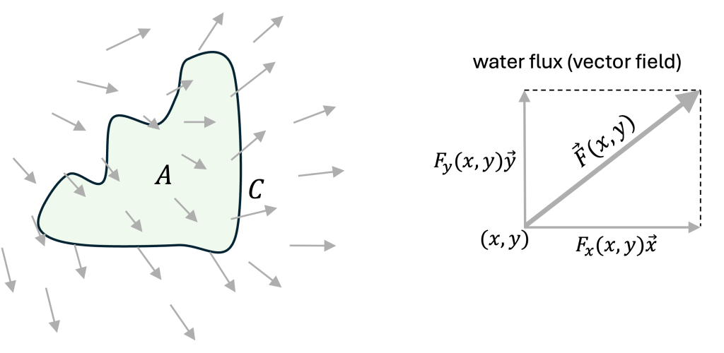
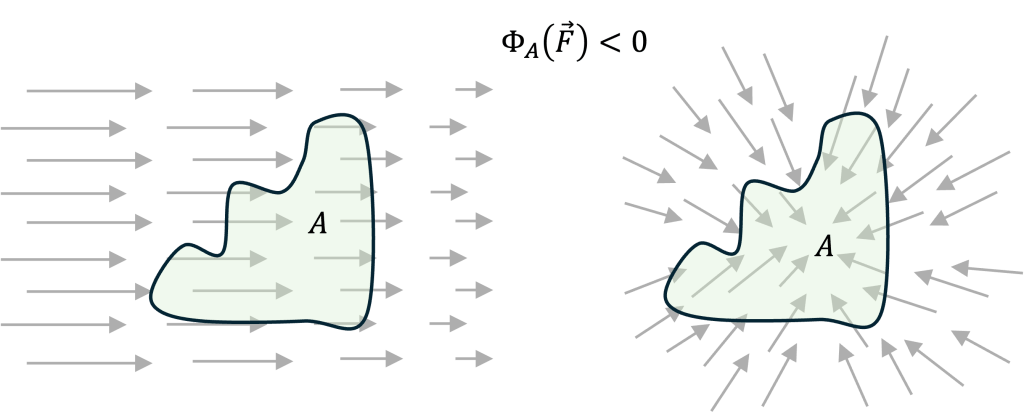
We then compute the net water flux, denoted as ${\Phi_A(\vec{F})}$ , as the outgoing flux minus the incoming flux through ${A}$ . We conclude that a leak is present within ${A}$ if ${\Phi_A(\vec{F})<0}$ :

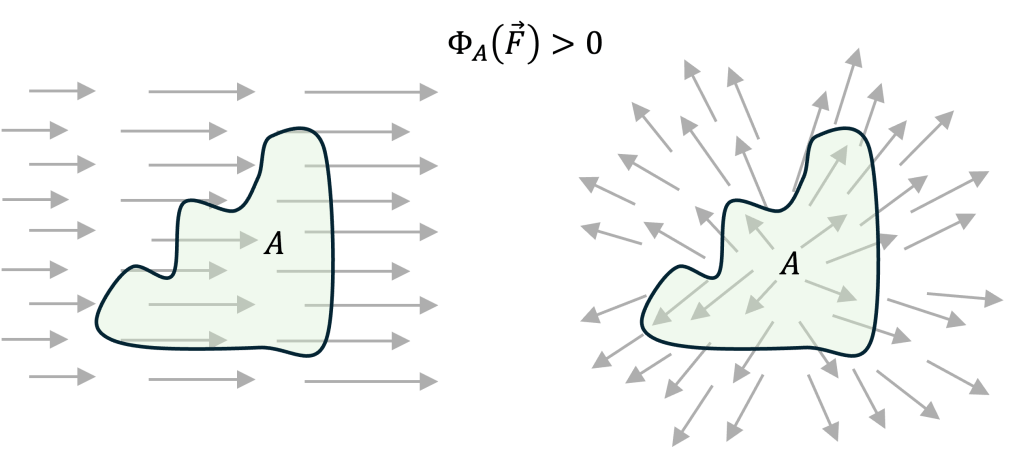
If, instead, the net flux is positive, a water source is detected:

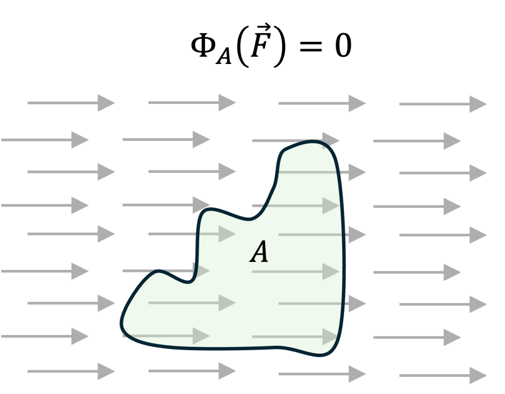
Else, if the flux is null, it means the water stream is conserved after flowing through ${A}$ :

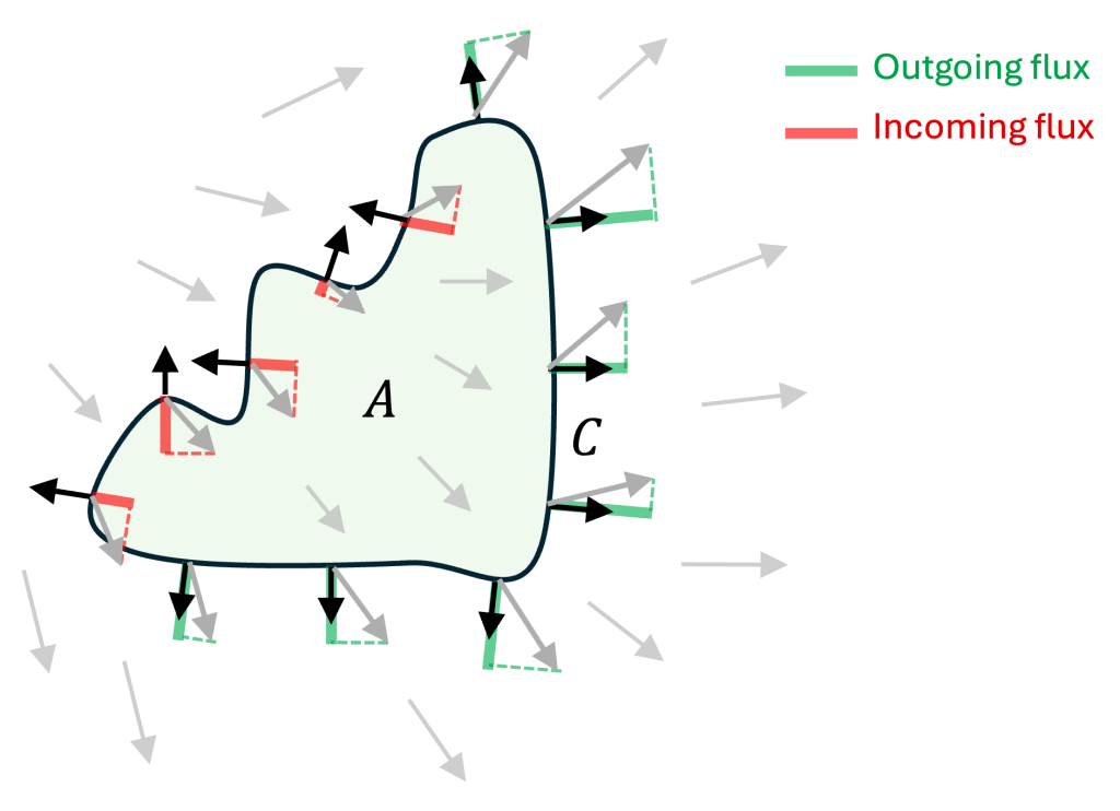
2. Net flux via a line integral

The net flux ${\Phi_A(\vec{F})}$ through ${A}$ can be computed as follows. Define ${C}$ as the contour of ${A}$ . At each point ${(x,y)}$ of ${C}$ , we evaluate the outgoing local flux in a small neighborhood of length ${dC}$ . This equals the scalar product between ${\vec{F}(x,y)}$ and the outward-pointing unitary vector ${\vec{n}(x,y)}$ perpendicular to ${C}$ , multiplied by ${dC}$ .

As intuition suggests, if ${\vec{F} \perp \vec{n}=0}$ then the local flux is null, while if ${\vec{F}}$ and ${\vec{n}}$ are anti-aligned then the outgoing flux is negative, i.e., incoming.

Finally, we sum up all local contributions along the contour. More compactly, this can be written as the line integral:

$\displaystyle \Phi_A(\vec{F}) := \int_{C} \left( \vec{F}(x,y) \cdot \vec{n}(x,y) \right) dC. \ \ \ \ \ (1)$

3. Net flux via the Divergence Theorem

The divergence theorem defines an equivalent method to compute the net water flux, as

$\displaystyle \Phi_A(\vec{F}) = \int \!\!\!\!\! \int_{A} (\nabla \cdot \vec{F}(x,y)) dA \ \ \ \ \ (2)$

where ${\nabla \cdot \vec{F}}$ is the divergence of ${\vec{F}}$ :

$\displaystyle \nabla \cdot \vec{F} (x,y) := \frac{d}{dx} F_x(x,y) + \frac{d}{dy} F_y(x,y) \ \ \ \ \ (3).$

Note that the cross-terms ${\frac{d}{dx} F_y(x,y)}$ and ${\frac{d}{dy} F_x(x,y)}$ do not intervene in the definition of divergence.

The divergence theorem is of practical importance because, among other things, the divergence integral is often easier to compute than the line integral since the former only entails scalar quantities.

In the following we provide an intuitive justification of (2), organized in four steps.

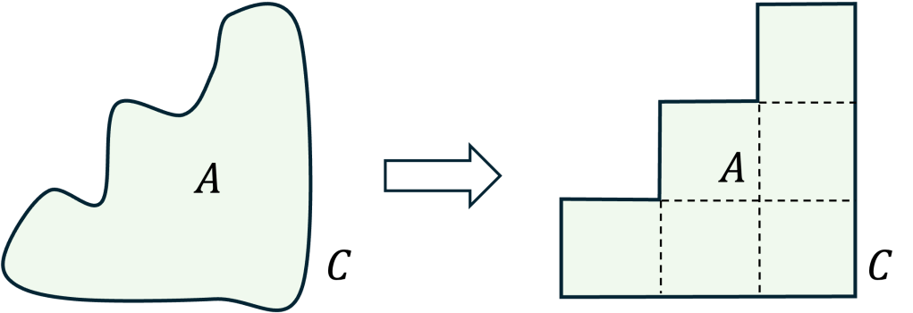
Step 1. We approximate the area ${A}$ as the collection of a myriad of small rectangles of side ${dx,dy}$ :

Step 2. We approximate the line integral on the ${i}$ -th rectangle by considering that the vector field remains constant along each (small) edge:

$\displaystyle \Phi_{A_i}(\vec F) \approx \vec{F}(x_i+dx, y_i) \cdot \vec{x} \, dy -\vec{F}(x_i,y_i) \cdot \vec{x} \, dy$

$\displaystyle \hspace{1cm} + \vec{F}(x_i,y_i+dy) \cdot \vec{y}\, dx - \vec{F}(x_i,y_i) \cdot \vec{y} \, dx \ \ \ \ \ (4)$

$\displaystyle = \frac{F_x(x_i+dx,y_i)-F_x(x_i,y_i)}{dx} dx \, dy + \frac{F_y(x_i,y_i+dy)-F_y(x_i,y_i)}{dy} dx \, dy \ \ \ \ \ (5)$

$\displaystyle \approx \left( \frac{d}{dx} F_x(x_i,y_i) + \frac{d}{dy} F_y(x_i,y_i) \right) dx \, dy \ \ \ \ \ (6)$

$\displaystyle := \left(\nabla \cdot \vec{F}(x_i,y_i)\right) dx \, dy \ \ \ \ \ (7)$

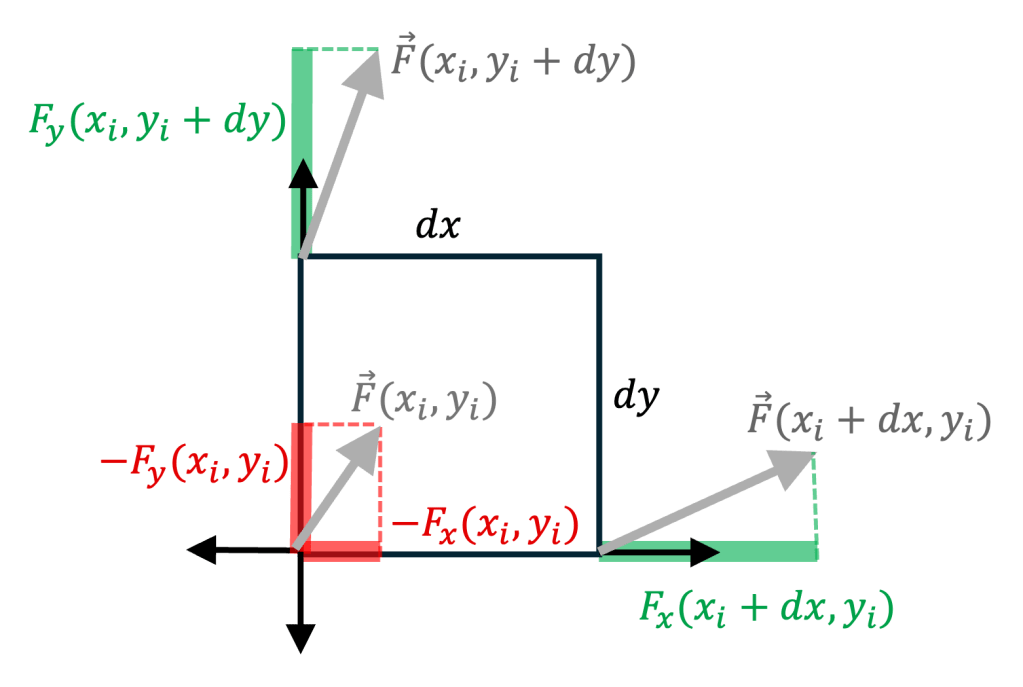
Interestingly, as a by-product, we have just heuristically shown that the divergence is effectively a measure of “net flux per unity of area”, i.e.,

$\displaystyle \nabla \cdot \vec{F}(x,y) = \lim_{A\rightarrow 0} \frac{\Phi_{A}(\vec F)}{A} \ \ \ \ \ (8)$

where the area ${A}$ encloses the point ${(x,y)}$ .

Step 3. When summing the net flux across all rectangles as ${\sum_i \Phi_{A_i}(\vec F)}$ , an interesting phenomenon occurs. In correspondence of adjacent rectangles, the normals at shared edges are oriented in opposite directions. As a result, the individual contributions of such edges to the line integral cancel each other out, leaving only the contributions from the boundary edges, which—aha!—lie along the contour ${C}$ .

Therefore, ${\sum_i \Phi_{A_i}(\vec F)}$ equals the net flux ${\Phi_A(\vec A)}$ , which by (7) also (approximately) coincides with the sum of the divergence contributions over the whole area ${A}$ :

$\displaystyle \Phi_A (\vec F) = \sum_i \Phi_{A_i}(\vec F) \approx \sum_i \left(\nabla \cdot \vec{F}(x_i,y_i) \right) dx \, dy. \ \ \ \ \ (9)$

Step 4. By letting the rectangle grid become infinitesimally fine, expression (9) tends to the original claim of the divergence theorem: ${\Phi_A(\vec{F}) = \int \!\!\!\!\! \int_{A} (\nabla \cdot \vec{F}(x,y)) dA}$ .

Posted

January 5, 2025

Calculus

Lorenzo Maggi

Tags:

divergence, divergencetheorem, flux, visual

Comments

4 responses to “The plumber’s secret weapon: The Divergence Theorem”

Alma

January 5, 2025

adesso non resta che trovare un idraulico nerd

LikeLike

Reply
H. Paul Keeler

January 20, 2025

Good presentation.

A similar style of proof (for the 2D version) is given in the book The Mathematical Mechanic by Mark Levi; see Section 7.3 – A Fluid Proof of Green’s Theorem.

When we were learning these calculus results at university, we were also learning electromagnetism that semester, so that somewhat muddied the waters in trying to understand the calculus. We should have used a fluid interpretation.

I guess one could say your argument holds water…

LikeLike

Reply
1. Lorenzo Maggi
  
  January 20, 2025
  
  Thanks, Paul, for the feedback!
  I wasn’t aware of this reference, and it’s reassuring to know that these intuitions aren’t entirely novel. 😊
  When drafting this post, I mainly relied on my memory of the topic and tried to present it in a way that would (hopefully) resonate with others.
  Thanks again!
  
  LikeLike
  
  Reply
H. Paul Keeler

January 20, 2025

You’re very welcome, Lorenzo.

I find your approach (much) more readable than what’s in the book. Your approach definitely resonates.

I am not sure if it’s a well-known book. I only recently picked up a secondhand copy, after hearing it mentioned somewhere.

All the best with future posts!

LikeLiked by 1 person

Reply

The plumber’s secret weapon: The Divergence Theorem

Share this:

Comments

4 responses to “The plumber’s secret weapon: The Divergence Theorem”

Leave a comment Cancel reply