Backpropagation

Chain rule to the rescue!

To train a deep neural network (DNN), one needs to repeatedly compute the gradient of the empirical loss with respect to all the DNN parameters ${\theta}$ . Since their number ${N^{\theta}}$ can be huge, it is crucial that the procedure for gradient computation grows “slowly” with ${N^{\theta}}$ . Back-propagation addresses this successfully by exploiting shrewdly the derivative chain rule, as we discuss in this post.

Supervised learning scenario. In supervised learning, the goal is to predict variable ${Y}$ from variable ${X}$ by training a model on a dataset ${\mathcal D}$ containing pairs of realizations ${(x,y)}$ of the aforementioned variables. Classically, the model is defined by a family of functions ${f(.,\theta)}$ parametrized by ${\theta}$ . Then, the empirical loss is minimized:

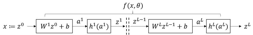
$\displaystyle \min_{\theta} \sum_{(x,y)\in \mathcal D} \frac{1}{2} \| f(x,\theta)-y\|^2:=\mathcal L(x,y,\theta). \ \ \ \ \ (1)$

Feed-forward DNN. We here consider that the model ${f(.\theta)}$ takes on the form of a feed-forward DNN, with ${L}$ fully connected hidden layers where each neuron is connected to all the neurons of the next layer.

We call the (column) vector ${x:=z^0=[z_i^0]_{i=1,\dots,M^0}}$ , which is multiplied by the ${M^1\times M^0}$ weight matrix ${W^1}$ and summed to the bias vector ${b^1}$ , to finally obtain the vector ${a^1}$ . Then, the non-linear (e.g., sigmoid) activation function ${h^1}$ , applied individually to each element of ${a^1}$ , produces the intermediate variable ${z^1}$ . The same procedure is iterated over all ${L}$ hidden layers as follows:

$\displaystyle z^{\ell} = h^{\ell} (a^{\ell}), \qquad \forall\, \ell=1,\dots,L \ \ \ \ \ (3)$

$\displaystyle a^{\ell} = W^{\ell} z^{\ell-1} + b^{\ell} \ \ \ \ \ (2)$

$\displaystyle z^{0} = x \ \ \ \ \ (4)$

where ${a^{\ell}\in \mathbb{R}^{M^\ell\times 1}}$ for all ${\ell}$ . We call ${f(.,\theta)}$ the function resulting from applying equations (2),(3) iteratively over all layers, where ${\theta=\{W^\ell,b^\ell\}_{1\le\ell\le L}}$ is the collection of all weights and biases. Hence, the DNN output produced by injecting ${x}$ as input is ${z^L=f(x,\theta)}$ .

Gradient of the loss. To minimize the loss ${\mathcal L(\theta)}$ via (any variant of) gradient descent, we must compute for each ${(x,y)}$ pair the gradient ${\nabla_{\theta}\mathcal L(x,y,\theta)}$ .

Finite difference? A (naive) option to compute the gradient ${\nabla_{\theta}\mathcal L(x,y,\theta)}$ is via finite difference:

$\displaystyle \nabla_{\theta} \mathcal L (x,y,\theta) \approx \left[\frac{\| f(x,\theta + \epsilon \delta^i)-y\|^2 - \| f(x,\theta)-y\|^2}{2\epsilon} \right]_{1\le i \le N^\theta} \ \ \ \ \ (5)$

where ${N^{\theta}}$ is the number of DNN parameters and ${\delta^i}$ is zero everywhere except for its ${i}$ -th element being 1.

Let us investigate the computation complexity of (5). Evaluating ${f_{\theta}(x)}$ requires to iterate (2) and (3) across all layers, each calling for ${N^{\theta}/L}$ and ${\sqrt{N^{\theta}/L}}$ basic operations (i.e., products, sums and computation of ${h}$ ). To compute the finite difference, such evaluation is then repeated ${2 N^{\theta}}$ times. Thus, the total complexity is in the order of

$\displaystyle (N^{\theta})^2 + N^{\theta}\sqrt{L N^{\theta}}.$

Since the number of parameters can be huge, a complexity quadratic in ${N^{\theta}}$ can be prohibitive. The natural question is: Can we do better? The answer is yes, as we show next.

Preliminaries: Jacobian matrix. Define the function ${\phi:\mathbb{R}^n\rightarrow \mathbb{R}^m}$ . The Jacobian of ${\phi}$ evaluated at ${x}$ is called ${J_\phi(x)}$ and is defined as:

$\displaystyle J_\phi(x) = \begin{bmatrix} \frac{\partial \phi_1}{\partial x_1}\big|_x & \dots & \frac{\partial \phi_1}{\partial x_n}\big|_x \\ \vdots & \ddots \vdots \\ \frac{\partial \phi_m}{\partial x_1}\big|_x & \dots & \frac{\partial \phi_m}{\partial x_n}\big|_x \end{bmatrix} \ \ \ \ \ (6)$

where ${\frac{\partial \phi_j}{\partial x_i}\big|_x}$ denotes the partial derivative of ${\phi_j}$ with respect to its ${i}$ -th input and evaluated at the point ${x}$ .

Observe that if ${\phi}$ is affine, i.e., ${\phi(x)=Wx+b}$ , where matrix ${W\in \mathbb R^{m\times n}}$ and column vector ${b\in \mathbb{R}^{m\times 1}}$ , then ${J_\phi(x)=W}$ .

If ${\phi}$ is separable across elements of ${x}$ , i.e., ${\phi_i(x)=\phi_i(x_i)}$ for all ${i}$ ‘s, then ${J_\phi(x)}$ is the diagonal matrix ${\mathrm{diag}(\phi'_i|_{x_i})_i}$ .

Preliminaries: Chain rule for derivative. Define two functions ${g:\mathbb{R}^n\rightarrow \mathbb{R}^m}$ and ${z:\mathbb{R}^m\rightarrow \mathbb{R}^l}$ and their composition ${\phi=z \circ g}$ , such that ${\phi(x)=z(g(x))}$ for all ${x\in \mathbb{R}^n}$ . If ${g}$ and ${z}$ are both unidimensional ( ${n=m=l=1}$ ), then

$\displaystyle \phi'|_x = z'|_{g(x)} g'|_x \ \ \ \ \ (7)$

In the general case, the derivative of the ${j}$ -th component of the composite function ${\phi=z\circ g}$ with respect to the ${i}$ -th input variable ${x_i}$ equals the sum over all intermediate functions ${g_k}$ of the individual contributions:

$\displaystyle \frac{\partial \phi_j}{\partial x_i}\Big|_x = \sum_{k=1}^{m} \frac{\partial z_j}{\partial g_k}\Big |_{g(x)} \frac{\partial g_k}{\partial x_i}\Big|_x , \quad \forall\, i,j. \ \ \ \ \ (8)$

More compactly, (8) can be rewritten as the product of the Jacobian’s of the individual functions:

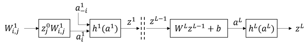
$\displaystyle J_{\phi}(x):=J_{z \circ g}(x) = J_{z}(g(x)) \cdot J_{g}(x). \ \ \ \ \ (9)$

Back-propagation (BP) rule. Our goal is to compute the derivative of the loss function with respect to any weight ${W_{i,j}^{\ell}}$ or any bias coefficient ${b_i^{\ell}}$ as efficiently as possible. We start by noticing that if ${W_{i,j}^{\ell}}$ changes then only ${a^{\ell}_i}$ changes at layer ${\ell}$ . By chain reaction, this modifies ${z^{\ell},a^{\ell+1},z^{\ell+1},\dots,z^L}$ and, finally, the loss ${\mathcal L}$ .

Hence, by chain rule:

$\displaystyle \frac{\partial \mathcal L}{\partial W_{i,j}^{\ell}}\Big|_{x,y,\theta} = \frac{\partial \mathcal L}{\partial a_{i}^{\ell}} \, \frac{\partial a_{i}^{\ell}}{\partial W_{i,j}^{\ell}}. \ \ \ \ \ (10)$

It stems from (2) that the second term is simply ${\frac{\partial a_{i}^{\ell}}{\partial W_{i,j}^{\ell}}=z_j^{\ell-1}}$ . Similarly, the derivative with respect to the bias term writes:

$\displaystyle \frac{\partial \mathcal L}{\partial b_{i}^{\ell}}\Big|_{x,y,\theta} = \frac{\partial \mathcal L}{\partial a_{i}^{\ell}} \, \frac{\partial a_{i}^{\ell}}{\partial b_{i}^{\ell}}. \ \ \ \ \ (11)$

where the second term ${\frac{\partial a_{i}^{\ell}}{\partial b_{i}^{\ell}}=1}$ .

Thus, to compute (10) and (11) we are left with evaluating ${\frac{\partial \mathcal L}{\partial a_{i}^{\ell}}}$ . By chain rule (9), the vector of partial derivatives ${\left[\frac{\partial \mathcal L}{\partial a_{i}^{\ell}}\right]_i:=\delta^\ell}$ , commonly referred to as the error term, can be computed as:

$\displaystyle \delta^\ell = J_{\mathcal L} \cdot J_{h^L} \cdot J_{W^L z^{L-1}+b^L} \cdot J_{h^{L-1}} \cdots J_{h^\ell} \ \ \ \ \ (12)$

where each term is calculated as follows:

$\displaystyle J_{\mathcal L}|_{z^L}=[(z^L_i-y_i)]_i.$

$\displaystyle J_{h^l}|_{a^{l}} = \mathrm{diag}(h'^l(a^l)), \qquad \forall\, l=\ell,\dots,L$

$\displaystyle J_{W^{l}z^{l-1}+b^{l}}|_{z^{l-1}}=W^l, \qquad \forall\, l=\ell,\dots,L$

The key observation is that the error term ${\delta^\ell}$ does not need to be recomputed from scratch at every layer. Rather, one can use an iterative computation with small incremental complexity, in a backward fashion from higher to lower layers.

Back-propagation procedure.

Forward: Compute the value of all the intermediate variables ${\{a^\ell,z^\ell\}_{1\le \ell\le L}}$ given the input ${x:=z^0}$ by evaluating (2),(3) at all layers.
Backward: For :
- If ${\ell=L}$ , then compute ${\delta^L = [(z^L_i-y_i)]_i \cdot \mathrm{diag}(h'^L(a^L))}$ .
  Else, compute incrementally ${\delta^{\ell} = \delta^{\ell+1} \cdot W^{\ell+1} \cdot \mathrm{diag}(h'^\ell(a^\ell))}$
- Compute ${\frac{\partial \mathcal L}{\partial W_{i,j}^{\ell}}=\delta_i^{\ell} z_j^{\ell-1}}$
- Set ${\frac{\partial \mathcal L}{\partial b_{i}^{\ell}}=\delta_i^{\ell}}$
Return ${\left\{\frac{\partial \mathcal L}{\partial W_{i,j}^{\ell}},\frac{\partial \mathcal L}{\partial b_{i}^{\ell}}\right\}_{i,j,\ell}}$ .

Complexity. As we showed before, evaluating the forward pass requires ${N^{\theta} + \sqrt{L N^{\theta}}}$ operations. Remarkably, the backward pass requires the same (order of) number of operations. This leads to an overall complexity being linear in the number of parameters ${N^{\theta}}$ , in contrast to the finite difference case, characterized by a quadratic complexity.

References.

[1] C. M. Bishop, H. Bishop. Deep Learning: Foundations and Concepts. Springer, 2024.

[2] I. Goodfellow, Y. Bengio, A. Courville. Deep learning. MIT Press, 2016.

[3] S.J. Prince (2023). Understanding Deep Learning. MIT press.

Backpropagation

Comments

Leave a comment Cancel reply

Backpropagation

Share this:

Comments

Leave a comment Cancel reply