The geometry of Gaussian variables

Gaussian (or normal) variables are all around the place. Their expressive power is certified by the Central Limit Theorem, stating that the mean of independent (and not necessarily Gaussian!) random variables tends to a Gaussian variable. And even when a variable is definitely not Gaussian, it is sometimes convenient to approximate it as one, via Laplace approximation, or to model it as a Gaussian mixture. Gaussian distributions also pop up, e.g., in Bayesian optimization, where an unknown function is modeled as a Gaussian process [1]. 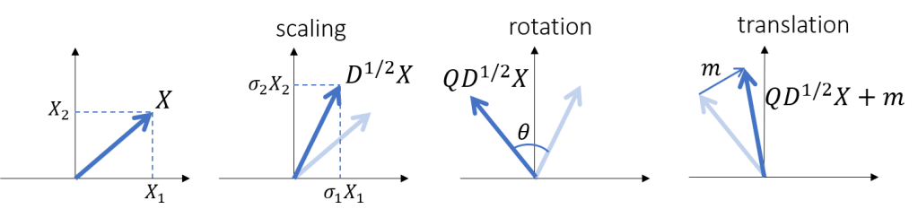And yet, while the uni-variate Gaussian case is simple to grasp (the “bell”!) and the expression of its density function is easy to remember (something like ${e^{-x^2}}$ …!), the multi-variate case is often perceived as more obscure and harder to visualize.

Geometric interpretation. In this post we try to shed some light on multi-variate Gaussian distributions case via a beautiful (and well known) geometric interpretation: any vector of jointly Gaussian variables can be obtained by applying basic geometric operations to a collection of independent standard normal variables (with zeros mean and unit variance), such as 1) scale 2) rotation and 3) translation.

How to read this post. To show that the geometric interpretation holds true we will take no shortcut, and delve first into a couple of preliminary concepts from calculus and linear algebra in Section 1. Yet, the hurried reader can jump directly to Section 2 where we serve the main dish with multi-variate Gaussian variables.

1. Some heavy-lifting warm-up

1.1. Change of variables in distributions

Let us first refresh our memory on calculus. Suppose we know the distribution ${f_X(.)}$ of a certain random variable ${X}$ . A second variable ${Y:=u(X)}$ is obtained from ${X}$ via a mapping ${u}$ .

We want to figure out the relationship between the distribution ${f_Y(.)}$ of ${Y}$ with the original one ${f_X(.)}$ . The following is a classic result from, e.g., [2].

Theorem 1 Let ${X}$ and ${Y}$ be multi-variate random variables with density function ${f_X(.)}$ and ${f_Y(.)}$ , respectively, such that ${Y=u(X)}$ . Suppose ${u(.)}$ differentiable and invertible, where ${u^{-1}(.):=v(.)}$ . Then,

$\displaystyle f_Y(y) = \left| \det \nabla_y v(y) \right| \times f_X(v(y)). \ \ \ \ \ (1)$

Let us inspect expression (1). Its latter term, ${f_X(v(y))}$ , is somehow expected: in analogy with discrete variables, the probability that ${Y=y}$ equals the probability that ${X}$ takes on the value that is mapped to ${y}$ via ${u}$ , namely ${X=v(y)}$ . For continuous variables, however, the density is not per se a probability, and the additional term ${\left| \det \nabla_y v(y) \right|}$ stems from the chain rule of derivatives. To convince ourselves that (1) holds true, it is useful to derive it in the uni-variate case. We call ${F_X}$ and ${F_Y}$ the cumulative distributions of ${X}$ and ${Y}$ , respectively. We need to distinguish between two cases, whether ${u}$ is i) increasing or ii) decreasing. (Note that ${u}$ is supposed to be invertible, hence there is no option iii)!)

If i) ${u}$ is increasing,

$\displaystyle \Pr(Y\le y) = \Pr\left(X\le v(y)\right) = F_X\left(v(y)\right). \ \ \ \ \ (2)$

To obtain ${f_Y(y):=\frac{d}{dy}F_Y(y)}$ we compute the derivative of the last expression with respect to ${y}$ :

$\displaystyle f_Y(y) = \frac{d}{dy} F_X\left(v(y)\right) = f_X\left( v(y) \right) \frac{d}{dy} v(y) \ \ \ \ \ (3)$

Else, if ii) ${u}$ is decreasing,

$\displaystyle \Pr(Y\le y) = \Pr\left(X\ge v(y)\right) = 1 - F_X\left(v(y)\right) \ \ \ \ \ (4)$

and

$\displaystyle f_Y(y) = \frac{d}{dy} \left[ 1- F_X\left(v(y)\right)\right] = -f_X\left( v(y) \right) \frac{d}{dy} v(y) \ \ \ \ \ (5)$

We observe that the two cases i) and ii) can be both written as

$\displaystyle f_Y(y) = f_X\left( v(y) \right) \left|\frac{d}{dy} v(y)\right| \ \ \ \ \ (6)$

since ${\frac{d}{dy} v(y)<0}$ if ${u}$ is decreasing. We finally notice that (6) is the uni-variate version of the seemingly daunting formula (1) in the multi-variate case!

1.2. Spectral decomposition of symmetric matrices

We now revise another fundamental result, on linear algebra this time: the spectral decomposition of symmetric real matrices, see [3].

Theorem 2 For all ${n\ge 1}$ , any symmetric matrix ${A\in \mathbb{R}^{n\times n}}$ can be written as the product ${Q D Q^T}$ , where ${Q}$ is real and unitary (i.e., its rows and columns are all orthogonal: ${QQ^T=Q^T Q=I}$ ) and ${D}$ is a diagonal matrix.

Proof: We split the proof in three parts: 1) ${A}$ has real eigenvalues, 2) ${A}$ has real eigenvectors, 3) the eigenvectors of ${A}$ are orthonormal.

Part 1: ${A}$ has real eigenvalues. If ${\lambda}$ is an eigenvalue of ${A}$ , then there exists a (eigen-)vector ${x}$ such that ${Ax=\lambda x}$ , which can be rewritten as ${\lambda=\frac{x^H A x}{x^H x}}$ , where ${.^H}$ denotes the Hermitian transpose. Its conjugate can be expressed as:

$\displaystyle \lambda^H = \frac{(x^H A x)^H}{x^H x} = \frac{x^H A^H x}{x^H x} = \frac{x^H A x}{x^H x} = \lambda \ \ \ \ \ (7)$

where we exploited the property ${(BC)^H=C^H B^H}$ for any matrices ${B,C}$ and the fact that ${A^H=A}$ since real symmetric.

Part 2:Each eigenvalue ${\lambda}$ of ${A}$ has a real eigenvector. Suppose that ${v=v^R+j v^I}$ is a complex eigenvector associated to ${\lambda}$ , namely ${Av=\lambda v}$ . Since ${A,\lambda}$ are real, then we can dissociate the expression into its real part ${Av^R=\lambda v^R}$ and imaginary part ${Av^I=\lambda v^I}$ . Then, ${v^R}$ and ${v^I}$ are both real eigenvectors with eigenvalue ${\lambda}$ . We have then proved that there exists a matrix ${Q}$ stacking the real eigenvectors of ${A}$ on its columns and a diagonal matrix ${D}$ collecting eigenvalues on the main diagonal such that ${A Q=Q D}$ . We still need to prove that ${Q}$ is unitary. Since ${Q^{-1}=Q^T}$ , we can also conclude that ${A=Q D Q^T}$ which will prove the thesis.

Part 3. ${Q}$ is unitary. We prove it by induction. Clearly, it holds for ${n=1}$ . Then, suppose that it holds for matrices ${A}$ of dimension ${n \times n}$ (then, ${A=Q D Q^T}$ ). Now, let ${\widetilde{A}}$ be of dimension ${(n+1)\times(n+1)}$ . Call ${v_1}$ one of its real eigenvectors, normalized such that ${v_1^T v_1=1}$ , with associated eigenvalue ${\lambda_1}$ . Then, we find ${n}$ column vectors ${[v_2,\dots,v_{n+1}]:=V}$ orthogonal with each other and also orthogonal with each other:

$\displaystyle V^T v = 0_n \ \ \ \ \ (8)$

To construct the matrix ${Q}$ that diagonalizes ${A}$ we first build in the following way. Since ${\widetilde{A}}$ is symmetric, ${V^T \widetilde{A} V}$ is also symmetric (in fact, ${(V^T \widetilde{A} V)^T=V^T \widetilde{A}^T V=(V^T \widetilde{A} V)}$ ). Then, by induction hypothesis, it can be decomposed as:

$\displaystyle \widetilde{Q} \widetilde{D} \widetilde{Q}^T = V^T \widetilde{A} V. \ \ \ \ \ (9)$

Lastly, we define ${Q}$ as ${[v_1, V\widetilde{Q}]}$ . Observe first that ${Q}$ is unitary, from (8). Then, compute:

$\displaystyle Q^T A Q = \begin{bmatrix} v_1^T \\ \widetilde{Q}^T V^T \end{bmatrix} \widetilde{A} \ [v_1, V\widetilde{Q}] =\begin{bmatrix} v_1^T Av_1^T & v_1^T AV\widetilde{Q} \\ \widetilde{Q}^T V^T A v_1 & \widetilde{Q}^T V^T AV\widetilde{Q} \end{bmatrix} \ \ \ \ \ (10)$

Let us first inspect the diagonal blocks. Since ${v_1}$ is a unitary eigenvector of ${A}$ , then ${v_1^T A v_1 =\lambda_1}$ . From (9) it stems that ${\widetilde{Q}^T V^T AV\widetilde{Q}=\widetilde{D}}$ . We now turn to the off-diagonal blocks, which are the same up to a transpose. Since ${v_1}$ is an eigenvector of ${A}$ , then ${\widetilde{Q}^T V^T A v_1=\lambda_1 \widetilde{Q}^T V^T v_1=0_n}$ via (8). Therefore, we conclude that

$\displaystyle A = Q \begin{bmatrix} \lambda_1 & 0_n^T \\ 0_n & \widetilde{D} \end{bmatrix} Q^T \ \ \ \ \ (11)$

which proves the thesis for matrices ${\widetilde{A}}$ of dimensions ${n+1}$ , and the theorem by induction process. $\Box$

1.3. Eigenvalues of positive semi-definite matrices

This third and last part of our warm-up section refines the result above for positive semi-definite matrices. A (real) matrix ${M}$ is positive semi-definite if ${x^T M x\ge 0}$ for all (real) vectors ${x}$ . Prominent examples are covariance matrices. In fact, consider any random vector ${X}$ and its covariance matrix ${C=\mathbb{E}[X-\mathbb{E}[X]] \mathbb{E}[X-\mathbb{E}[X]]^T}$ . Then, we realize that

$\displaystyle x^T C x=x^T \mathbb{E}[X-\mathbb{E}[X]] \mathbb{E}[X-\mathbb{E}[X]]^T x \ \ \ \ \ (12)$

$\displaystyle \quad = (\mathbb{E}[X-\mathbb{E}[X]]^T x)^2\ge 0, \quad \forall\, x \ \ \ \ \ (13)$

We next show that, if the symmetric matrix ${A}$ in Theorem 2 is positive semi-definite, then the diagonal matrix ${D}$ has non-negative values on its main diagonal, see [3]. This result will serve us well in Section 2 where ${D}$ carries variances on its diagonal, which clearly cannot be negative.

Theorem 3 The eigenvalues of a symmetric positive semi-definite matrix are all non-negative.

Proof: We compute ${x^T A x}$ for a semi-definite matrix ${A\in \mathbb R^{n\times n}}$ . It stems from Theorem 2 that we can write ${A=QD Q^T=\sum_i \sigma_i q_i q_i^T}$ , where ${q_i}$ is the ${i}$ -th column of ${Q}$ . Since ${q_1,\dots,q_n}$ are ${n}$ independent vectors (in fact, ${Q}$ is invertible!), they form a basis of ${\mathbb R^n}$ . Therefore, ${x}$ itself can be written as a linear combination of vector ${q}$ ‘s, i.e., ${x=\sum_{i=1}^n \alpha_i q_i}$ . Hence,

$\displaystyle x^T A x = \left(\sum_{i=1}^n \alpha_i q_i^T \right) \left(\sum_{i=1}^n \sigma_i q_i q_i^T\right) \left(\sum_{i=1}^n \alpha_i q_i \right) \ \ \ \ \ (14)$
By the orthogonality property of ${q}$ ‘s ( ${q_i^T q_j=0}$ for ${i\ne j}$ , ${q_i^T q_i=1}$ for all ${i}$ ),

$\displaystyle x^T A x = \left(\sum_{i=1}^n \alpha_i q_i^T \right) \left(\sum_{i=1}^n \sigma_i \alpha_i q_i \right) = \sum_{i=1}^n \alpha_i^2 \sigma_i. \ \ \ \ \ (15)$

By hypothesis, ${\sum_{i=1}^n \alpha_i^2 \sigma_i\ge 0}$ . Since this must hold for all ${x}$ (hence, for all ${\{\alpha_i\}_i}$ ), then ${\sigma_i\ge 0}$ for all ${i}$ , which proves the thesis. $\Box$

2. The main dish: Gaussian variables

After such a warm-up, we can address the main topic of this post: multi-variate Gaussian variables. Next we show the two-way relationship between independent and correlated Gaussian variables:

independent ${\rightarrow}$ correlated: by scaling, rotating and translating independent standard (i.e., with zero mean and unit variance) Gaussian variables we still obtain Gaussian variables, correlated with each other (Section 2.1)
correlated ${\rightarrow}$ independent: any vector of correlated Gaussian variables can be interpreted as the result of appropriate scale, rotation and translation operations applied to independent standard Gaussian variables (Section 2.2).

2.1. From independent standard to correlated Gaussian variables

Consider a list ${X=[X_1,\dots,X_n]}$ of ${n}$ independent standard Gaussian variables (i.e., with zero mean and unit variance). Recall the (marginal) probability density function (pdf) of each individual ${X_i}$ :

$\displaystyle f_{X_i}(x_i) = (2\pi)^{-\frac{1}{2}} \exp\left( -\frac{x_i^2}{2} \right), \qquad \forall\, i. \ \ \ \ \ (16)$
Since all variables are independent, the multi-variate pdf of the whole vector ${X}$ is simply the product of the individual pdfs:

$\displaystyle f_{X}(x) = \prod_i f_{X_i}(x_i) = (2\pi)^{-\frac{n}{2}} \exp{-\frac{x^T x}{2}} \ \ \ \ \ (17)$

To spice things up, let us transform ${X}$ into a more expressive random vector ${Y}$ , via basic operations such as:

scale, obtained by multiplying each ${X_i}$ by a positive scalar ${\sigma_i}$ (this is without loss of generality: ${\sigma_i X_i}$ and ${-\sigma_i X_i}$ have the same distribution!). In matricial form, the result of scale is ${D^{-\frac{1}{2}} X}$ , where ${D^{-\frac{1}{2}}}$ is a diagonal matrix carrying ${\sigma_i}$ ‘s over the main diagonal (note that the exponent ${1/2}$ will come in handy in the following);
rotation, resulting from multiplying the scaled vector ${D^{-\frac{1}{2}} X}$ by a rotation, or unitary, matrix ${Q}$ , such that ${Q^TQ=QQ^T=I}$ . In two dimensions ( ${n=2}$ ), $\displaystyle Q=\begin{bmatrix} \cos \theta & -\sin \theta \\ \sin \theta & \cos \theta \end{bmatrix}. \ \ \ \ \ (18)$
We will see that these first two operations introduce correlation across different elements of the random vector ${Y}$ ;
translation, by simply adding a constant offset ${\mu}$ to the scaled and rotated vector ${QD X}$ .

The resulting random vector ${Y}$ writes:

$\displaystyle Y=QD^{\frac{1}{2}} X + \mu \ \ \ \ \ (19)$

To compute the pdf of ${Y}$ we can apply Theorem 1 on change of variables. But before, we still need to:

compute the inverse function ${v(.)}$ , mapping ${Y}$ to ${X}$ . Fortunately, this is easy algebra: $\displaystyle v(Y)=D^{-\frac{1}{2}} Q^T(Y-\mu) \ \ \ \ \ (20)$
compute the determinant of the Jacobian ${\nabla_y v(y)=D^{-\frac{1}{2}} Q^T}$ . By exploiting the property ${\det(AB)=\det(A)\det(B)}$ we deduce that: $\displaystyle |\det \nabla_y v(y)|=|\det(D^{-\frac{1}{2}})\det\left(Q^T\right)| = |\det (D^{-\frac{1}{2}})| \ \ \ \ \ (21)$
where the last expression stems from ${\det (Q)=\pm 1}$ (in fact, ${QQ^T=I}$ , hence ${(\det Q)^2=1}$ ).

We can finally exploit Theorem 1 to transform the pdf of the independent standard variables ${X}$ , in Equation (17), into the pdf of the transformed variable ${Y}$ :

$\displaystyle f_Y(y) = \left| \det \nabla_y v(y) \right| \times f_X(v(y)) \ \ \ \ \ (22)$

$\displaystyle \qquad = (2\pi)^{-\frac{n}{2}} |\det(D^{-\frac{1}{2}})| \exp\left[ \left(D^{-\frac{1}{2}} Q^T(y-\mu)\right)^T D^{-\frac{1}{2}} Q^T(y-\mu) \right] \ \ \ \ \ (23)$

$\displaystyle \qquad = (2\pi)^{-\frac{n}{2}} |\det(D^{-\frac{1}{2}})| \exp\left[ (y-\mu)^T Q D^{-1} Q^T(y-\mu) \right] \ \ \ \ \ (24)$

We reached our goal but we are quite not satisfied yet: the last formula does not look like what we usually find in textbooks, e.g., [1]. Let us then conveniently define the matrix ${\Sigma}$ as:

$\displaystyle \Sigma = Q D Q^T \ \ \ \ \ (25)$

$\displaystyle \Sigma^{-1} = Q D^{-1} Q^T \ \ \ \ \ (26)$

After realizing that ${|\det(D^{-\frac{1}{2}})|=|\det(\Sigma^{-\frac{1}{2}})|}$ , we finally get to the classic expression of multi-variate Gaussian variables:

$\displaystyle f_Y(y) = (2\pi)^{-\frac{n}{2}} |\det(\Sigma^{-\frac{1}{2}})| \exp\left[ (y-\mu)^T \Sigma^{-1} (y-\mu) \right]. \ \ \ \ \ (27)$

The vector ${\mu}$ and the matrix ${\Sigma}$ carry two key pieces of information on ${Y}$ , namely its mean vector and covariance matrix, respectively. In fact,

$\displaystyle \mathbb{E} [Y] = \mathbb{E}[QD^{\frac{1}{2}}X+\mu] = QD^{\frac{1}{2}}\mathbb{E}[X]+\mu=\mu \ \ \ \ \ (28)$

$\displaystyle \mathbb{E}\left[(Y-\mu)(Y-\mu)^T\right] = \mathbb{E}\left[ Q D^{\frac{1}{2}} X X^T (D^{\frac{1}{2}})^T Q^T \right] \ \ \ \ \ (29)$

$\displaystyle \qquad = Q D^{\frac{1}{2}} \mathbb{E}\left[ X X^T\right] D^{\frac{1}{2}} Q^T = Q D Q^T=\Sigma. \ \ \ \ \ (30)$

since ${\mathbb{E}[X]=0}$ and ${\mathbb{E}[ X X^T]=I}$ .

2.2. From correlated to independent standard Gaussian variables

In this last section we take the reverse path and, given a vector of Gaussian variables ${Y}$ with mean ${\mu}$ and covariance matrix ${\Sigma}$ , we want to retrieve (if any!) the basic operations (scaling, rotation and translation) that led from independent normal variables ${X}$ to the correlated ${Y}$ . To this aim, all ingredients are there: it suffices to invoke Theorem 2 and decompose ${\Sigma}$ as ${Q D Q^T}$ , where as usual ${Q}$ is a unitary matrix and ${D}$ is diagonal. Then, Theorem 3 informs us that ${D}$ carries non-negative number on its diagonals, hence ${D^{\frac{1}{2}}}$ is well defined and real. Thus, previous Section 2 tells us that ${Y}$ can be interpreted as the scaling by ${D^{\frac{1}{2}}}$ , rotation by ${Q}$ and translation by ${\mu}$ of a set of independent normal Gaussian variables ${X}$ .

Take-home message: Suppose you are given a set of Gaussian variables ${Y}$ with a certain covariance matrix ${\Sigma}$ and mean ${\mu}$ . To gain precious geometric intuitions, decompose ${\Sigma=Q D Q^T}$ to retrieve the scale (via ${D}$ ) and rotation (via ${Q}$ ) operations that connect ${Y}$ with a simple vector of independent standard variables!

References

[1] Bishop, C. (2006). Pattern recognition and machine learning. Springer.
[2] Billingsley, P. (2017). Probability and measure. John Wiley & Sons.
[3] Strang, G. (2022). Introduction to linear algebra. Wellesley-Cambridge Press.

The geometry of Gaussian variables

Comments

Leave a comment Cancel reply

The geometry of Gaussian variables

Share this:

Comments

Leave a comment Cancel reply